The Riemann integral
Part 7 · Integrals · Chapter 1 · Lecture notes, volume 7 (PDF) · Exercises, volume 7 (PDF) · Exercises: Riemann integral and properties · Slides (PDF) · App: Riemann sums
Prerequisites
-
From this module, «Ordered fields, supremum/infimum and the completeness axiom»: supremum and infimum of a set and their existence in \(\R\).
-
From this module, «Summations, geometric and arithmetic progressions»: the summation symbol and the sum of the first \(n\) natural numbers.
-
From this module, «Continuous functions» and «Weierstrass theorem and intermediate value theorem»: continuity, maximum and minimum on a closed and bounded interval, intermediate values.
Objectives
At the end of this chapter you will be able to:
-
compute the lower and upper sums of a bounded function with respect to a partition;
-
state the definition of the Riemann integral and interpret it as a signed area;
-
prove that monotone functions and continuous functions on \([a,b]\) are integrable;
-
use linearity, additivity, monotonicity and the inequality \(\left|\int_a^b f\right| \le \int_a^b |f|\);
-
state and prove the integral mean value theorem.
1. Partitions and Riemann sums
Definition 1: partition of an interval
Given an interval \([a,b]\), with \(a<b\), a partition of \([a,b]\) is a finite set of points
The points \(x_k\) divide \([a,b]\) into the \(n\) intervals \(I_k = [x_{k-1}, x_k]\), with \(k \in \{1, 2, \dots, n\}\), of length \(\Delta x_k = x_k - x_{k-1}\).
-
The partition is called uniform when all the intervals have the same length \(\Delta x_k = \frac{b-a}{n}\), that is, when \(x_k = a + k\,\frac{b-a}{n}\).
-
If \(P \subseteq P'\), the partition \(P'\) is called finer than \(P\) (or a refinement of \(P\)): it is obtained from \(P\) by adding points.
Definition 2: lower sum and upper sum
Let \(f:[a,b] \rr \R\) be a bounded function and let \(P = \{x_0, x_1, \dots, x_n\}\) be a partition of \([a,b]\). Setting, for every \(k \in \{1, 2, \dots, n\}\),
the lower sum and the upper sum of \(f\) with respect to \(P\) are the numbers
-
The bounds \(m_k\) and \(M_k\) are real numbers because \(f\) is bounded. Since \(m_k \le M_k\) for every \(k\), we always have \(s(f,P) \le S(f,P)\).
-
If \(f \ge 0\), the lower sum is the area of the rectangles inscribed in the region under the graph, the upper sum that of the circumscribed rectangles.
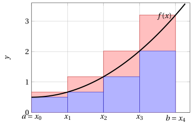
- In the figure, with \(f\) increasing, the blue rectangles form the lower sum and the blue rectangles together with the red ones the upper sum: the area under the graph lies in between.
Example 1: lower and upper sums of \(f(x)=x\)
Let \(f(x) = x\) on \([0,1]\) and let \(P_n\) be the uniform partition with \(x_k = \frac{k}{n}\). Since \(f\) is increasing, on every interval \(I_k\) the minimum is at the left endpoint and the maximum at the right endpoint:
With the sum of the first \(n\) natural numbers, \(\sum_{k=1}^{n} k = \frac{n(n+1)}{2}\), we get
The difference \(S(f,P_n) - s(f,P_n) = \frac{1}{n}\) tends to \(0\) and both sums tend to \(\frac12\).
Proposition 1: sums and refinements
Let \(f:[a,b] \rr \R\) be bounded. If \(P'\) is finer than \(P\), then
Proof
It is enough to consider the case in which \(P'\) has one more point, \(y \in (x_{k-1}, x_k)\): the general case follows by adding one point at a time. The two sums differ only on the interval \(I_k\), which in \(P'\) is split into \([x_{k-1}, y]\) and \([y, x_k]\).
The infimum over a subset is greater than or equal to the infimum over the whole set, hence
Consequently
that is, \(s(f,P') \ge s(f,P)\). For the upper sums we argue in the same way with the suprema, which over a subset are smaller than or equal: \(S(f,P') \le S(f,P)\). □
Corollary 1
Let \(f:[a,b] \rr \R\) be bounded. For every pair of partitions \(P_1\) and \(P_2\) of \([a,b]\) we have
Proof
The partition \(P = P_1 \cup P_2\) is finer than both \(P_1\) and \(P_2\). By the Proposition on sums and refinements
□
-
Every upper sum is therefore an upper bound of the set of lower sums. By the completeness axiom the following exist and are finite:
\[ \sup_{P} s(f,P) ~~\le~~ \inf_{P} S(f,P) \]where supremum and infimum are taken over all partitions \(P\) of \([a,b]\).
2. The Riemann integral
Definition 3: Riemann integrable function
A bounded function \(f:[a,b] \rr \R\) is called Riemann integrable on \([a,b]\) if
The common value is called the integral of \(f\) on \([a,b]\) and is denoted by
-
The function \(f\) is called the integrand, the numbers \(a\) and \(b\) are the limits of integration.
-
The variable \(x\) is a dummy variable: \(\int_a^b f(x)\,dx\), \(\int_a^b f(t)\,dt\) and \(\int_a^b f(u)\,du\) denote the same number.
-
The symbol \(\int\) is an elongated \(S\) (sum) and \(dx\) recalls the widths \(\Delta x_k\) of the rectangles.
2.1 Geometric interpretation
-
If \(f \ge 0\) on \([a,b]\), the integral is the area of the region under the graph (the subgraph)
\[ T_f = \big\{ (x,y) \in \R^2 : a \le x \le b, ~ 0 \le y \le f(x) \big\} \]which lies between the inscribed rectangles (lower sums) and the circumscribed ones (upper sums).
-
If \(f\) changes sign, the parts below the \(x\)-axis count with a minus sign: the integral is a signed area, that is, the area above the axis minus the area below the axis.
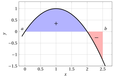
- In the figure the integral of \(f\) on \([a,b]\) is the blue area minus the red area.
Example 2: integral of a constant
Let \(f(x) = c\) on \([a,b]\), with \(c \in \R\). For every partition \(P\) we have \(m_k = M_k = c\), hence
The constant function is integrable and
If \(c>0\) this is the area of the rectangle with base \(b-a\) and height \(c\).
Example 3: integral of \(f(x)=x\)
Let us go back to \(f(x) = x\) on \([0,1]\) and to the uniform partitions \(P_n\) of the Example on the lower and upper sums of \(f(x)=x\). For every \(n\)
Letting \(n \rr \ip\) both ends tend to \(\frac12\), hence
This is the area of the triangle with vertices \((0,0)\), \((1,0)\) and \((1,1)\).
Example 4: integral of \(f(x)=x^2\)
Let \(f(x) = x^2\) on \([0,1]\) and \(P_n\) the uniform partition. The function is increasing on \([0,1]\), so \(m_k = \left(\frac{k-1}{n}\right)^2\) and \(M_k = \left(\frac{k}{n}\right)^2\). Using the formula \(\sum_{k=1}^{n} k^2 = \frac{n(n+1)(2n+1)}{6}\) (it is proved by induction) we get
Both tend to \(\frac{2}{6} = \frac13\) as \(n \rr \ip\); arguing as in the previous example
Example 5: a non-integrable function
The Dirichlet function on \([0,1]\) is
Every interval \(I_k\) contains both rational and irrational numbers (density of \(\Q\) and of \(\R \setminus \Q\) in \(\R\)), so \(m_k = 0\) and \(M_k = 1\) for every \(k\). For every partition
Hence \(\sup_P s(D,P) = 0 \neq 1 = \inf_P S(D,P)\): the Dirichlet function is bounded but it is not Riemann integrable.
2.2 Integrability criterion
Theorem 1: Riemann's integrability criterion
A bounded function \(f:[a,b] \rr \R\) is integrable on \([a,b]\) if and only if for every \(\varepsilon > 0\) there exists a partition \(P\) of \([a,b]\) such that
Proof
Let \(I_- = \sup_P s(f,P)\) and \(I^+ = \inf_P S(f,P)\); we know that \(I_- \le I^+\).
-
(\(\Leftarrow\)) For every \(\varepsilon > 0\) there is \(P\) with \(s(f,P) \le I_- \le I^+ \le S(f,P)\) and \(S(f,P) - s(f,P) < \varepsilon\). Hence \(0 \le I^+ - I_- < \varepsilon\) for every \(\varepsilon > 0\), that is, \(I^+ = I_-\).
-
(\(\Rightarrow\)) Let \(I = I_- = I^+\) and let \(\varepsilon > 0\). By the properties of supremum and infimum there exist \(P_1\) and \(P_2\) with
\[ s(f,P_1) > I - \frac{\varepsilon}{2} {\rm ~~~~and~~~~} S(f,P_2) < I + \frac{\varepsilon}{2} \]With \(P = P_1 \cup P_2\), by the Proposition on sums and refinements, \(S(f,P) - s(f,P) \le S(f,P_2) - s(f,P_1) < \varepsilon\).
□
2.3 Riemann sums
-
Choosing a point \(t_k\) in each interval \(I_k\), the sum \(\sigma(f,P) = \sum_{k=1}^{n} f(t_k)\,\Delta x_k\) is called a Riemann sum.
-
Since \(m_k \le f(t_k) \le M_k\), we have \(s(f,P) \le \sigma(f,P) \le S(f,P)\): if \(f\) is integrable and \(S(f,P) - s(f,P) \rr 0\), the Riemann sums tend to the integral too, whatever the choice of the points \(t_k\).
-
For continuous functions with uniform partitions, \(t_k\) can be the left endpoint, the right endpoint or the midpoint of \(I_k\): this is how an integral is approximated on a computer.
Try it — the interactive graph below shows what you have just read: move the sliders.
3. Classes of integrable functions
Theorem 2: integrability of monotone functions
If \(f:[a,b] \rr \R\) is monotone, then \(f\) is integrable on \([a,b]\).
Proof
Assume \(f\) non-decreasing (the non-increasing case is analogous). The function is bounded, because \(f(a) \le f(x) \le f(b)\). Let \(P_n\) be the uniform partition, with \(\Delta x_k = \frac{b-a}{n}\). On every interval \(I_k\) we have \(m_k = f(x_{k-1})\) and \(M_k = f(x_k)\), hence
because the sum telescopes. Given \(\varepsilon > 0\), it is enough to take \(n > \frac{(b-a)(f(b) - f(a))}{\varepsilon}\) to get \(S(f,P_n) - s(f,P_n) < \varepsilon\). By Riemann's integrability criterion, \(f\) is integrable. □
- A monotone function may have discontinuity points: for example the integer part \([x]\) is integrable on every interval \([a,b]\), even though it has a jump at every integer.
3.1 Uniform continuity
Definition 4: uniformly continuous function
A function \(f: I \rr \R\) is called uniformly continuous on the interval \(I\) if for every \(\varepsilon > 0\) there exists \(\delta > 0\) such that
-
In continuity at every point the number \(\delta\) may depend on the point; in uniform continuity the same \(\delta\) works for all the points of \(I\).
-
A function that is uniformly continuous on \(I\) is continuous at every point of \(I\).
Example 6: uniform continuity
The function \(f(x) = x^2\) is uniformly continuous on \([0,1]\): for \(x, y \in [0,1]\)
and it is enough to choose \(\delta = \frac{\varepsilon}{2}\).
The function \(g(x) = \frac{1}{x}\) is continuous on \((0,1]\) but not uniformly continuous: the points \(x_n = \frac1n\) and \(y_n = \frac{1}{n+1}\) have distance \(\frac{1}{n(n+1)} \rr 0\), while \(|g(x_n) - g(y_n)| = 1\) for every \(n\).
Theorem 3: Heine–Cantor theorem
If \(f:[a,b] \rr \R\) is continuous on the closed and bounded interval \([a,b]\), then \(f\) is uniformly continuous on \([a,b]\).
Proof
By contradiction: there exists \(\varepsilon > 0\) such that for every \(n \ge 1\) there are \(x_n, y_n \in [a,b]\) with
The sequence \(\{x_n\}\) is bounded. By the Bolzano–Weierstrass theorem (every bounded sequence has a convergent subsequence: it is proved with the same bisection used for the Weierstrass theorem) there exists a subsequence \(x_{n_j} \rr c\), with \(c \in [a,b]\) because the interval is closed.
Since \(|x_{n_j} - y_{n_j}| < \frac{1}{n_j}\), also \(y_{n_j} \rr c\). By the continuity of \(f\) at \(c\)
which contradicts \(|f(x_{n_j}) - f(y_{n_j})| \ge \varepsilon\) for every \(j\). □
3.2 Integrability of continuous functions
Theorem 4: integrability of continuous functions
If \(f:[a,b] \rr \R\) is continuous, then \(f\) is integrable on \([a,b]\).
Proof
By the Weierstrass theorem \(f\) is bounded. Let \(\varepsilon > 0\). By the Heine–Cantor theorem there exists \(\delta > 0\) such that
Take a partition \(P\) with all intervals of length \(\Delta x_k < \delta\). On every \(I_k\), by the Weierstrass theorem, \(f\) has a minimum \(m_k = f(\xi_k)\) and a maximum \(M_k = f(\eta_k)\), with \(|\xi_k - \eta_k| \le \Delta x_k < \delta\). Hence \(M_k - m_k < \frac{\varepsilon}{b-a}\) and
By Riemann's integrability criterion, \(f\) is integrable. □
Remark 1
One can prove that a function which is bounded on \([a,b]\) and continuous except at finitely many points is integrable as well. Moreover, changing an integrable function at finitely many points gives an integrable function with the same integral.
4. Properties of the integral
-
It is convenient to extend the integral symbol to the case of equal or swapped limits:
\[ \int_a^a f(x)\,dx = 0 {\rm ~~~~and~~~~} \int_b^a f(x)\,dx = -\int_a^b f(x)\,dx \]
4.1 Linearity
Theorem 5: linearity of the integral
If \(f\) and \(g\) are integrable on \([a,b]\) and \(\alpha, \beta \in \R\), then \(\alpha f + \beta g\) is integrable on \([a,b]\) and
Proof
It is enough to treat separately the sum \(f+g\) and the multiple \(\alpha f\).
-
Sum. On every interval \(I_k\) we have \(\inf (f+g) \ge \inf f + \inf g\) and \(\sup (f+g) \le \sup f + \sup g\), hence
\[ s(f,P) + s(g,P) \le s(f+g,P) \le S(f+g,P) \le S(f,P) + S(g,P) \]Given \(\varepsilon > 0\), by Riemann's integrability criterion and the Proposition on sums and refinements there is a partition \(P\) (the union of those that work for \(f\) and for \(g\)) with \(S - s < \frac{\varepsilon}{2}\) both for \(f\) and for \(g\). Then \(S(f+g,P) - s(f+g,P) < \varepsilon\) and \(f+g\) is integrable. Moreover \(\int (f+g)\) and \(\int f + \int g\) both lie between \(s(f,P)+s(g,P)\) and \(S(f,P)+S(g,P)\): their distance is less than \(\varepsilon\) for every \(\varepsilon > 0\), so they coincide.
-
Multiple. If \(\alpha \ge 0\), then \(\inf (\alpha f) = \alpha \inf f\) and \(\sup (\alpha f) = \alpha \sup f\), hence \(s(\alpha f, P) = \alpha\, s(f,P)\) and \(S(\alpha f,P) = \alpha\, S(f,P)\). If \(\alpha < 0\), infimum and supremum are swapped: \(s(\alpha f,P) = \alpha\, S(f,P)\) and \(S(\alpha f,P) = \alpha\, s(f,P)\). In both cases \(\int \alpha f = \alpha \int f\).
□
4.2 Additivity with respect to the interval
Theorem 6: additivity with respect to the interval
Let \(a < c < b\). A function \(f\) is integrable on \([a,b]\) if and only if it is integrable on \([a,c]\) and on \([c,b]\), and in that case
Proof
By the Proposition on sums and refinements we may use only partitions \(P\) of \([a,b]\) containing \(c\) (adding \(c\) does not increase the difference \(S - s\)). Such a \(P\) is the union of a partition \(P_1\) of \([a,c]\) and a partition \(P_2\) of \([c,b]\), and
Hence \(S(f,P) - s(f,P)\) is the sum of the two differences, both non-negative: it is smaller than \(\varepsilon\) if and only if both are (up to halving \(\varepsilon\)). By Riemann's integrability criterion the two integrability conditions are equivalent. Finally \(\int_a^b f\) and \(\int_a^c f + \int_c^b f\) both lie between \(s(f,P)\) and \(S(f,P)\), whose distance is less than \(\varepsilon\): they coincide. □
- With the convention on swapped limits, the additivity formula holds for \(a\), \(b\), \(c\) in any order, provided that \(f\) is integrable on the largest interval.
Example 7: additivity
Let \(f(x) = x\) for \(x \in [0,1]\) and \(f(x) = 1\) for \(x \in [1,3]\). The function is continuous, hence integrable, and by additivity
where we used the Example on the integral of \(f(x)=x\) and the one on the integral of a constant.
4.3 Monotonicity and absolute value
Theorem 7: monotonicity of the integral
If \(f\) and \(g\) are integrable on \([a,b]\) and \(f(x) \le g(x)\) for every \(x \in [a,b]\), then
Proof
On every interval \(I_k\) we have \(\inf f \le \inf g\), hence \(s(f,P) \le s(g,P) \le \int_a^b g\) for every partition \(P\). Taking the supremum over \(P\), \(\int_a^b f = \sup_P s(f,P) \le \int_a^b g\). □
Corollary 2: estimates of the integral
Let \(f\) be integrable on \([a,b]\).
-
If \(f(x) \ge 0\) for every \(x \in [a,b]\), then \(\int_a^b f(x)\,dx \ge 0\).
-
If \(m \le f(x) \le M\) for every \(x \in [a,b]\), then
\[ m\,(b-a) \le \int_a^b f(x)\,dx \le M\,(b-a) \]
Proof
Apply the theorem on the monotonicity of the integral comparing \(f\) with the constants \(0\), \(m\) and \(M\), whose integrals are given by the Example on the integral of a constant. □
Example 8: an estimate without computing the integral
On \([0,1]\) the function \(f(x) = e^{-x^2}\) is decreasing, so \(e^{-1} \le f(x) \le 1\). By the Corollary on the estimates of the integral
even though \(e^{-x^2}\) has no elementary antiderivative.
Theorem 8: integral of the absolute value
If \(f\) is integrable on \([a,b]\), then \(|f|\) is integrable on \([a,b]\) too and
Proof
-
Integrability of \(|f|\). For \(x, y \in I_k\) we have \(\big| |f(x)| - |f(y)| \big| \le |f(x) - f(y)| \le M_k - m_k\). Taking the supremum in \(x\) and the infimum in \(y\), the difference between the supremum and the infimum of \(|f|\) on \(I_k\) is at most \(M_k - m_k\). Hence \(S(|f|,P) - s(|f|,P) \le S(f,P) - s(f,P)\) and we conclude with Riemann's integrability criterion.
-
Inequality. From \(-|f(x)| \le f(x) \le |f(x)|\), by the linearity and the monotonicity of the integral,
\[ -\int_a^b |f(x)|\,dx \le \int_a^b f(x)\,dx \le \int_a^b |f(x)|\,dx \]which is the claim.
□
Example 9: the inequality can be strict
Let \(f(x) = x\) on \([-1,1]\). The signed areas of the two triangles cancel out, while for \(|x|\) they add up:
Hence \(\left|\int_{-1}^1 x\,dx\right| = 0 < 1 = \int_{-1}^1 |x|\,dx\).
5. Integral mean value theorem
Definition 5: integral mean
Let \(f\) be integrable on \([a,b]\). The integral mean (or mean value) of \(f\) on \([a,b]\) is the number
- If \(f \ge 0\), the integral mean is the height of the rectangle with base \([a,b]\) having the same area as the region under the graph of \(f\).
Theorem 9: integral mean value theorem
If \(f:[a,b] \rr \R\) is continuous, then there exists \(c \in [a,b]\) such that
Proof
By the Weierstrass theorem \(f\) has a minimum \(m\) and a maximum \(M\) on \([a,b]\). By the Corollary on the estimates of the integral
The integral mean is therefore a value between the minimum and the maximum of \(f\). By the intermediate value theorem \(f\) takes all values between \(m\) and \(M\): there exists \(c \in [a,b]\) at which \(f(c)\) equals the integral mean. □
Example 10: integral mean of \(x^2\)
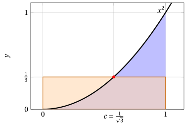
By the Example on the integral of \(f(x)=x^2\), the integral mean of \(x^2\) on \([0,1]\) is
The point of the integral mean value theorem is found by solving \(c^2 = \frac13\) with \(c \in [0,1]\): \(c = \frac{1}{\sqrt3}\). In the figure the orange rectangle of height \(\frac13\) has the same area as the blue region under the parabola.
Remark 2
The continuity assumption cannot be dropped. The function \(f(x) = 0\) for \(x \in [0,1)\) and \(f(x) = 1\) for \(x \in [1,2]\) is integrable (it is monotone) and, by additivity and the Remark on changes at finitely many points, its integral mean is \(\frac12 \int_0^2 f(x)\,dx = \frac12\), a value that \(f\) does not take.
6. In summary
In summary
-
For a bounded function and a partition of \([a,b]\), the lower sum uses the infima and the upper sum the suprema; refining the partition the former increases and the latter decreases.
-
\(f\) is integrable if the supremum of the lower sums equals the infimum of the upper sums; equivalently, if \(S(f,P) - s(f,P)\) can be made arbitrarily small.
-
If \(f \ge 0\) the integral is the area under the graph; in general it is a signed area.
-
Monotone functions and continuous functions on \([a,b]\) are integrable (for continuous ones we need the Heine–Cantor theorem); the Dirichlet function is not.
-
The integral is linear, additive with respect to the interval and monotone, and \(\left|\int_a^b f\right| \le \int_a^b |f|\).
-
A continuous function takes its integral mean at least at one point of \([a,b]\).
Exercises on this chapter: Riemann integral and properties