Weierstrass theorem and intermediate value theorem

Part 3 · Limits of functions and continuity · Chapter 9 · lecture notes by Fabio Furini · Chapter PDF

1. Weierstrass theorem

• The following theorem establishes sufficient but not necessary conditions for a function to have a maximum and a minimum.

Theorem 1: Weierstrass theorem

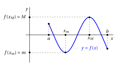
If a function \(f: [a,b] \rr \R\) is continuous on the interval \([a,b]\), then it has a maximum \(M\) and a minimum \(m\) in \([a,b]\).

Under the hypotheses of the theorem there exist:

\[ x_m {\rm ~~and~~} x_M \in [a, b] {\rm ~~~~such~that~~~~} f(x_m) \le f(x) \le f(x_M) {\rm ~~~for~every~~~} x \in [a, b] \]

We say that \(x_m\) is a minimum point of \(f\) and \(m = f (x_m)\) is the minimum of \(f\).

We say that \(x_M\) is a maximum point of \(f\) and \(M = f (x_M)\) is the maximum of \(f\).

Properties of the supremum/infimum

• Given two non-empty subsets \(E_1\), \(E_2\) of \(\R\) we have:

  \[ \sup \big(E_1 \cup E_2 \big) = \max \big(\sup E_1, \sup E_2 \big) \]

  This property holds for both bounded and unbounded sets. If one or both sets are unbounded above we have: \(\sup (E_1 \cup E_2) = \ip\). For the infimum we have:

  \[ \inf \big(E_1 \cup E_2 \big) = \min \big(\inf E_1, \inf E_2 \big) \]

Proof

We prove that \(f\) has a maximum in \([a, b]\). Consider the function:

\[ f : [a, b] \rr \R, {\rm ~~~and~set~~~~} \ell = \sup_{[a,b]} f \]

We now need to prove that:

• \(i)\) \(\ell\) is finite, that is, \(\ell \in \R\);

• \(ii)\) \(\ell\) is equal to \(f(x_0)\) for some \(x_0\in [a,b]\) (and hence \(\ell\) is the maximum and \(x_0\) is the maximum point).

We split the interval \([a, b]\) into two equal intervals: \(I_{1}\) and \(I_{2}\); by the properties of the supremum we have:

\[ \sup_{[a,b]} f = \max \bigg( \sup_{I_{1}} f, \sup_{I_{2}} f \bigg) {\rm ~~~that~is~~~} \sup_{[a,b]} f = \sup_{I_{1}} f {\rm ~~~or~~~} \sup_{[a,b]} f = \sup_{I_{2}} f \]

Hence for one of the two intervals, which we call \([a_1, b_1]\), it will be true that:

\[ \ell = \sup_{[a_1,b_1]} f \]

We now split \([a_1 , b_1]\) into two equal intervals; for one of them, which we call \([a_2, b_2]\), it will be true that:

\[ \ell = \sup_{[a_2,b_2]} f \]

Proceeding by bisection in this way, we construct a sequence of intervals \([a_n, b_n]\), each contained in the previous ones, with the properties:

1. the sequence \(\{a_n\}\) is monotone increasing and bounded, and the sequence \(\{b_n\}\) is monotone decreasing and bounded;

2. \(b_n - a_n = \frac{b-a}{2^n} \rr 0 {\rm~~as~~} n \rr \ip;\)

3. \(\displaystyle \ell = \sup_{[a_n,b_n]} f\) (the supremum of \(f\) is attained in the interval \([a_n,b_n]\))

By the same reasoning used in the proof of the intermediate zero theorem (which uses the monotonicity theorem for sequences), from points 1) and 2) it follows that the sequences \(\{a_n\}\) and \(\{b_n\}\) converge to the same limit \(x_0 \in [a, b]\):

\[ a_n \rr x_0 {\rm ~~and~~} b_n \rr x_0 {\rm ~~as~~} n \rr \ip. \]

We now proceed by cases. □

Proof

Case 1: \(\ell \in \R\)

If \(\ell \in \R\), for every \(n\) there exists a point \(t_n \in [a_n, b_n]\) such that:

\[\begin{equation} \label{RRRR} \ell - \frac{1}{n} < f(t_n) \le \ell \end{equation}\]

Indeed, since \(\ell - \frac{1}{n}\) is less than \(\ell\), which is the least upper bound of the values of \(f(x)\) in \([a_n, b_n]\), \(\ell - \frac{1}{n}\) is not an upper bound; hence there exists \(t_n \in [a_n, b_n]\) with property \(\eqref{RRRR}\).

Since \(t_n \in [a_n, b_n]\), and we have:

\[ a_n \rr x_0 {\rm ~~and~~} b_n \rr x_0 {\rm ~~as~~} n \rr \ip {\rm ~~~then~~~}t_n \rr x_0 {\rm ~~as~~} n \rr \ip \]

by the comparison (squeeze) theorem. Again by the comparison theorem, \(\eqref{RRRR}\) then gives

\[ \lim_{n \rr \ip} f(t_n) = \ell \]

On the other hand, since \(f\) is continuous and \(t_n \rr x_0\), we have:

\[ \lim_{n \rr \ip} f(t_n) = f(x_0) {\rm ~~~~therefore~~~~} f(x_0) = \ell. \]

Then, since \(\ell\) is the \(\sup\) of the values of \(f\) in \([a, b]\), \(\ell\) is the maximum of \(f\) in \([a, b]\), and it is attained at the point \(x_0\), the maximum point. Therefore, in this case the theorem is proved.

Case 2: \(\ell = \ip\)

If \(\ell = \ip\), for every \(n\) there exists a point \(t_n \in [a_n,b_n]\) such that:

\[\begin{equation} \label{RRRRR} f (t_n) \ge n \end{equation}\]

Reasoning as above, one proves that \(t_n \rr x_0\) for some \(x_0 \in [a, b]\). Since \(f\) is continuous at \(x_0\):

\[ \lim_{n \rr \ip} f(t_n) = f (x_0) \]

but by \(\eqref{RRRRR}\) we have

\[ \lim_{n \rr \ip} f(t_n) = \ip \]

which is a contradiction, since at \(x_0\) the function must have a finite value. Hence this case cannot occur.

Similarly, one proves that the function has a minimum in \([a, b]\). □

The proof is a constructive existence proof (similar to that of the intermediate zero theorem), which, however, cannot be used algorithmically since, after each bisection, it is not known a priori which interval the supremum or infimum is associated with.

The hypotheses of the Weierstrass theorem are all essential

1. The interval must be closed

   Consider as a counterexample:

   \[ f(x) = x {\rm ~~with~~} x \in (0,1) \]

   The function is continuous on a bounded, but not closed, interval. In this case, the function has neither a maximum nor a minimum (its supremum, \(1\), and its infimum, \(0\), are not attained by the function).

2. The interval must be bounded

   Consider as a counterexample:

   \[ f(x) = x {\rm ~~with~~} x \in \R \]

   The function is continuous on an unbounded interval but has neither a maximum nor a minimum (it is not even bounded).

3. The function must be continuous

   Consider as a counterexample:

   \[ f(x) = \begin{cases} x & {\rm ~~for~~} x \in (0,1)\\ \frac{1}{2} & {\rm ~~for~~} x=0 {\rm ~~and~~} x=1 \end{cases} \]

   The function is defined on a closed and bounded interval \([0, 1]\) but it is not continuous. The function has neither a maximum nor a minimum (its supremum, \(1\), and its infimum, \(0\), are not attained by the function).

2. Intermediate value theorem

Theorem 2: Intermediate value theorem

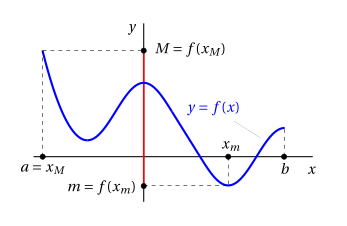
If a function \(f: [a,b] \rr \R\) is continuous on \([a,b]\), then it has a maximum \(M\) and a minimum \(m\) in \([a,b]\) and it takes all the values between \(m\) and \(M\).

We are under the hypotheses of the Weierstrass theorem, hence we have:

\[ x_m {\rm ~~and~~} x_M \in [a, b] {\rm ~~~~such~that~~~~} f(x_m) \le f(x) \le f(x_M) {\rm ~~~for~every~~~} x \in [a, b] \]

The intermediate value theorem further tells us that:

\[ \forall \lambda \in (m,M), {\rm ~~~there~exists~~~} x(\lambda) \in [x_m,x_M] {\rm ~~such~that~~} f\big(x(\lambda)\big) = \lambda \]

This property is called the intermediate value property.

Proof

From the Weierstrass theorem we have a maximum point \(x_{M}\) and a minimum point \(x_m\) such that \(f(x_M)=M\) (maximum) and \(f(x_m)=m\) (minimum) in \([a,b]\). Let

\[ m < \lambda < M \]

and consider the function

\[ g(x) = f(x) - \lambda {\rm ~~with~~} x \in [x_m,x_M] \]

which is continuous since \(f(x)\) is continuous on \([a,b]\) and \(x_m, x_M \in [a,b]\).

Hence:

\[ g(x_M) = f(x_M) -\lambda = M -\lambda >0 \]

\[ g(x_m) = f (x_m) -\lambda = m -\lambda < 0 \]

Then, by the intermediate zero theorem, there exists \(x(\lambda) \in (x_m,x_M)\) such that:

\[ g\big(x(\lambda)\big) = 0 {\rm ~~~~that~is~~~~} f\big(x(\lambda)\big) = \lambda \]

□

• Given a function continuous on an interval \([a,b]\), graphically we have:

!!! esempio "Example 1: Discontinuous function without the intermediate value property"

Consider for example the graph of the following function, discontinuous on $[a,b]$:

![Figure 3](../img/limits-09-weierstrass/fig03.svg){ .fig .ovale loading=lazy style="width:85%" }

This function does not have the intermediate value property, that is, the values $\lambda \in (y_1,y_2)$ are not outputs of $f$.

• The properties of the two previous theorems can be summarized in the following single statement:

Corollary 1

If \(f: [a, b] \rr \R\) is continuous, then

\[ f([a, b]) = [m, M]; \]

i.e., the image of an interval \([a, b]\) is the interval with endpoints:

\[ \displaystyle m = \min_{[a,b]} f {\rm ~~~and~~} M = \max_{[a,b]} f. \]

Proof

It follows from the Weierstrass theorem and the intermediate value theorem. □

Example 2: Failure of the intermediate value theorem in \(\Q\)

• Let

  \[ f(x) = x^2 \]

  and consider \(f\) as a function from the set \(\Q\) of rational numbers to \(\Q\) itself (this is legitimate because the square of a rational number is rational).

• Then f does not have the intermediate value property.

• Indeed, for example,

  \[ f (1) = 1, f(2) = 4, \]

  but \(f\) does not take all the rational values between 1 and 4: for example, it never takes the value 2, or 3.

• In other words, the intermediate value property holds for continuous functions thanks to the properties of the set of real numbers.

• This is a further reason why it is useful to work in the set of real numbers rather than in the set of rational numbers.

3. Existence theorem for the \(n\)-th root

Theorem 3

For every \(y \in \R\), \(y > 0\) and \(n \in \N\), \(n \ge 1\), there exists one and only one \(x \in \R, x >0\), such that \(x^n = y\).

This number \(x\) is called the \(n\)-th root of \(y\)

Proof

Consider the function \(f (x) = x^n\).

This function is continuous on all of \(\R\), because it is the product of \(n\) continuous functions \(g (x) = x\).

We show that there exist

\[ x_2 > x_1 > 0 {\rm ~~such~that~~} x_1^n < y < x_2^n. \]

If \(y=1\) the \(n\)-th root exists and is unique; moreover:

1. If \(y > 1\): it suffices to choose

   \[ x_1 = 1, x_2 = y {\rm ~~and~we~have~~} x_1^n < y < x_2^n ~~~(1 < y < y^n) \]

2. If \(y < 1\): it suffices to choose

   \[ x_1 = y, x_2 = 1 {\rm ~~and~we~have~~} x_1^n < y < x_2^n ~~~(y^n< y < 1 ) \]

Then we can apply the intermediate value theorem to the continuous function \(f(x) = x^n\) on the interval \([x_1, x_2]\). Here its minimum is \(x_1^n\) and its maximum is \(x_2^n\).

Since:

\[ x_1^n < y < x_2^n, {\rm ~~there~exists~~} x_0 \in [x_1,x_2] {\rm ~~such~that~~} x_0^n = y. \]

Uniqueness follows from the fact that the function is strictly increasing. □