Vibration phenomena
Part 2 · Functions · Chapter 6 · lecture notes by Fabio Furini · Chapter PDF
1. Vibration phenomena
-
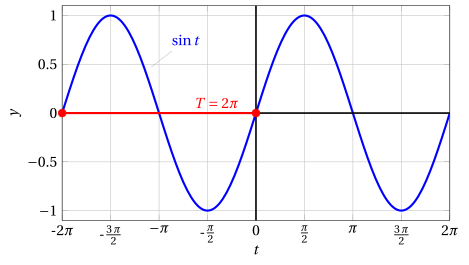
We have seen that the sine and cosine functions are periodic with period \(2\: \pi\). We will use the variable \(t\) to denote time.
-
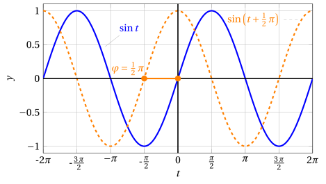
Recall that \(\sin (t + \varphi)\) corresponds to a phase shift \(\varphi\) (horizontal translation).
The functions:
where \(a\), \(b\) and \(\omega\) are positive real numbers, are called elementary vibrations. They are periodic functions with
Example 1: period
For example, considering \(t' = t + \frac{2\: \pi}{\omega}\):
-
Clearly we have:
\[ |a\: \sin \:(\omega \: t)| \le a \qquad{\rm ~~and~~}\qquad |b\: \cos \:(\omega \: t)| \le b \]
The functions \(\eqref{trig_vibr}\) describe elementary vibrations characterized by
also called angular velocity, which indicates how many periods there are in an interval of length \(2\: \pi\). Moreover, they are characterized by the
which indicates how many times the function repeats itself in an interval of length \(1\)
Example 2: of amplitude, angular frequency and frequency
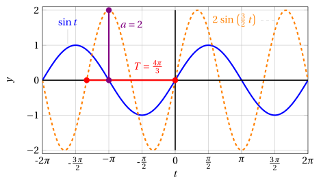
The angular frequency \(\omega=\frac{3}{2}\) means that there are 1.5 periods in an interval of length \(2 \: \pi\). The frequency \(\nu\) is \(\frac{3}{4\:\pi}\).
-
The function
\[\begin{equation} \label{EEE} h(t) = a\: \sin \:(\omega \: t) + b\: \cos \:(\omega \: t) \end{equation}\]describes the superposition of the two elementary vibrations with the same angular frequency \(\omega\). The latter is again an elementary vibration, phase-shifted with respect to the previous ones.
-
Indeed, setting
\[ A= \sqrt{a^2 + b^2} \]we can write
\[\begin{equation} \label{EEEE} h(t) = A \: \underbrace{\frac{a}{ \sqrt{a^2 + b^2}}}_{\alpha} \: \sin \:(\omega \: t) + A \: \underbrace{\frac{b}{ \sqrt{a^2 + b^2}}}_{\beta} \: \cos \:(\omega \: t) \end{equation}\] -
Now observe that the numbers
\[ \alpha=\frac{a}{ \sqrt{a^2 + b^2}} {\rm ~~and~~} \beta=\frac{b}{ \sqrt{a^2 + b^2}} \]satisfy the conditions
\[ -1 \le \alpha \le 1 \qquad -1 \le \beta \le 1 \qquad \alpha^2 + \beta^2=1 \]Hence there exists a unique angle \(\varphi\) such that
\[ \cos \varphi = \alpha \qquad \sin \varphi = \beta \]so that \(\eqref{EEEE}\) can be rewritten in the following form
\[\begin{align} \label{EEEEE} h(t) & = A \: \cos \varphi \: \sin (\omega \:t) + A \: \sin \varphi \: \cos (\omega \:t)\nonumber\\[2ex] & = A \: \sin (\omega\:t + \varphi) \end{align}\]Therefore \(h(t)\) represents an elementary vibration with amplitude \(A\), angular frequency \(\omega\), phase-shifted by an angle \(\varphi\).
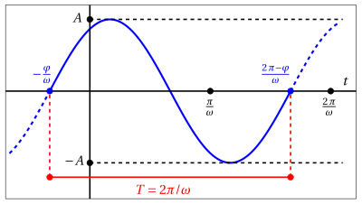
In summary:
- Under fairly general conditions, a periodic natural phenomenon can be written as the superposition of a finite or infinite number of elementary vibrations with different frequencies (Fourier series).
Try it — the interactive graph below shows what you have just read: move the sliders.
2. Damping and amplification effects
- By multiplying an elementary vibration by powers or exponentials, we can model damping or amplification effects.
First example
-
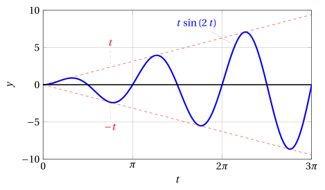
For example, consider the function
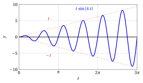
\[ h(t) = t \: \sin \:(\omega \: t) \]which models an amplified vibration.
-
Since \(-1 \le \sin \:(\omega \: t) \le 1\), we have
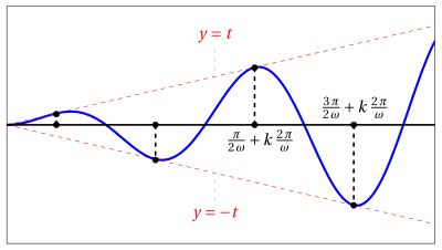
\[ -t \le t \: \sin \:(\omega \: t) \le t \]and hence the graph of \(h(t)\) lies between the graphs of the lines with equations \(y = -t\), \(y = t\).
-
At the points where
\[ \sin \:(\omega\:t) = 1 \]i.e.,
\[ t = \frac{\pi}{2 \: \omega} + k \: \frac{2\:\pi}{\omega} \qquad (k=0,1,2,\dots) \]the graph of \(h(t)\) touches that of \(y=t\).
-
At the points where
\[ \sin \:(\omega\:t) = -1 \]i.e.,
\[ t = \frac{3\: \pi}{2 \: \omega} + k \: \frac{2\:\pi}{\omega} \qquad (k=0,1,2,\dots) \]the graph of \(h(t)\) touches that of \(y=-t\).
-
From the graph we can see that multiplication by \(t\) has the effect of amplifying the vibration as \(t\) increases.
Second example
-
For example, consider the function
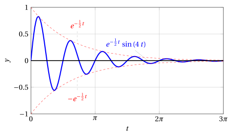
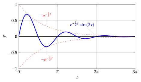
\[ k(t) = e^{-\alpha\:t} \: \sin \:(\omega \: t) \qquad (\alpha > 0) \]which models a damped vibration.
-
Recalling that
\[ e^{-\alpha\:t} = \left(\frac{1}{e^{\alpha}}\right)^t \]is an exponential with base less than \(1\), considerations analogous to those made for the function \(h(t)\) show that the graph of \(k\) lies between the graphs of the functions
\[ y_1 = e^{-\alpha\:t} {\rm ~~~~and~~~~} y_2 = -e^{-\alpha\:t} \]as shown in the figure: