Inverse functions
Part 2 · Functions · Chapter 11 · lecture notes by Fabio Furini · Chapter PDF
1. Invertible functions and inverse functions
-
Given a real function of a real variable \(f : D \rightarrow \mathbb{R}\), for every input \(x\) in the domain \(D\) there exists a unique output \(y=f(x)\) in the image of the domain \(f(D)\).
-
If, in addition, for every output \(y = f(x) \in f(D)\) there exists a unique input \(x \in D\), then \(f\) is called invertible, and it establishes a one-to-one correspondence between the domain \(D\) of \(f\) and the image of the domain \(f(D)\).
Definition 1: of invertible function
A function \(f : D \rightarrow \mathbb{R}\) is invertible on the domain \(D\) if one of the following equivalent conditions holds:
that is, if \(f\) is injective.
WARNING: the definition of invertible function given here for real functions of a real variable is different from the usual one given for functions between arbitrary sets, which also requires surjectivity. In this case injectivity is enough because we define the inverse on the image of \(f\) and not on its whole codomain.
Definition 2: of inverse function
Given an invertible function \(f : D \rightarrow \mathbb{R}\), the function that associates to each output \(y \in f(D)\) the unique input \(x \in D\) such that \(f(x) = y\) is called the inverse function of \(f\) and is denoted by the symbol \(f^{-1}\).
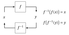
The pair \(f\) and \(f^{-1}\) is written as:
The black box of \(f^{-1}\) works backwards with respect to that of \(f\), according to the following scheme:
The invertibility condition is equivalent to requiring that the graph of \(f\) be intersected in at most one point by every line parallel to the \(x\)-axis.
Example 1: graph of an invertible function
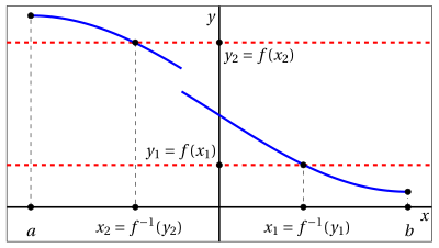
Graph of a function that is invertible on \([a,b]\), since every line parallel to the \(x\)-axis either does not intersect the graph of \(f\) or intersects it in exactly one point.
Example 2: graph of a non-invertible function
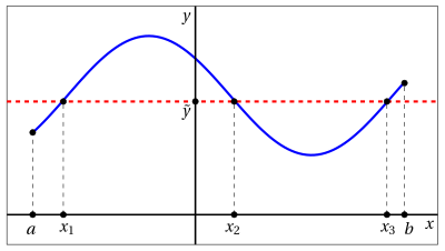
Graph of a function that is not invertible on \([a,b]\), since for the indicated value \(\tilde{y}\) there are several values \(x\) (precisely \(x_1\) , \(x_2\) and \(x_3\)) whose image is \(\tilde{y}\).
Theorem 1
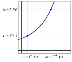
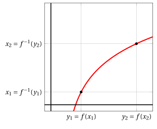
If a function \(f : D \rightarrow \mathbb{R}\) is strictly increasing (decreasing) on \(D\), then it is invertible on \(D\). Moreover, its inverse function is strictly increasing (decreasing).
For the strictly increasing case, graphically we have:
Proof
Consider the case of a function that is strictly increasing on \(D\) and two arbitrary values \(x_1, x_2 \in D\) (the strictly decreasing case is analogous).
If \(x_1 \neq x_2\), then either \(x_1 < x_2\) or \(x_1 > x_2\). Since \(f\) is strictly increasing, we have:
In both cases \(f(x_1) \neq f(x_2)\), therefore \(f\) is invertible.
Consider the inverse function \(f^{-1}\), that is, \(x = f^{-1} (y)\), and let us prove that it is strictly increasing. Consider two arbitrary values \(y_1, y_2 \in f(D)\), with \(y_1 < y_2\).
If we had \(f^{-1}(y_1) =x_1 \ge x_2= f^{-1}(y_2)\), since \(f\) is strictly increasing we would have \(y_1 = f(x_1) \ge f(x_2) =y_2\), that is, \(y_1 \ge y_2\). This cannot happen, since it contradicts \(y_1 < y_2\) (contradiction).
Consequently, we have \(f^{-1}(y_1) =x_1 < x_2= f^{-1}(y_2)\), that is, \(f^{-1} (y_1) < f^{-1}(y_2)\), and hence \(f^{-1}\) is strictly increasing. □
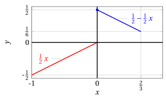
However, a function can be invertible even without being strictly increasing or decreasing.
Example 3: invertible function that is neither strictly increasing nor strictly decreasing
For example, the following piecewise-defined function is invertible:
-
Two classes of functions that are certainly not invertible are:
-
even (symmetric) functions, since:
\[ f(-x) = f (x) \] -
periodic functions, since:
\[ f(x + T) =f(x) \]
-
1.1 Graph of the inverse function
-
The relations between an invertible function \(f\) and its inverse function \(f^{-1}\):
\[\begin{equation*} f: \begin{cases} y = f(x)\\ x \in D \end{cases} ~~~~~~~~ f^{-1}: \begin{cases} x = f^{-1}(y)\\ y \in f(D) \end{cases} \end{equation*}\]indicate that if the point \((x_0, y_0)\) lies on the graph of \(f\), then the point \((y_0, x_0)\) lies on the graph of \(f^{-1}\).
-
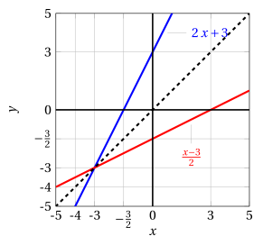
Since the points \((x_0, y_0)\) and \((y_0, x_0)\) are symmetric with respect to the bisector with equation \(y = x\), the graph of \(f^{-1}\) is obtained from that of \(f\) by symmetry with respect to the bisector.
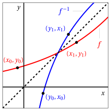
If the analytic expression of \(f\) is known and \(f\) is invertible, the analytic expression of \(f^{-1}\) is found by trying to solve for \(x\) the equation:
Note that it is not always possible to find it, even in cases where the inverse function exists!
Given \(a,b \in \R, a \neq 0\), we have:
Example 4: inverse function of an affine function
The function \(f: \mathbb{R} \rightarrow \mathbb{R}, x \mapsto 2 \: x +3\) is strictly increasing, hence invertible on \(\mathbb{R}\), and the equation
gives for \(f^{-1}\) the analytic expression:
that is, the function: \(f^{-1}: \mathbb{R} \rightarrow \mathbb{R}, y \mapsto \frac{y-3}{2}\).
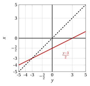
The graphs \(y=2 \: x +3\) and \(y=\frac{x-3}{2}\) are symmetric with respect to the bisector \(y = x\)
We have:
Example 5: inverse function of \(f(x)=x^2\)
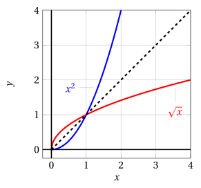
The function \(f: \mathbb{R} \rightarrow \mathbb{R}, x \mapsto x^2\) is strictly increasing on the interval \([0,+\infty)\), hence invertible there; the equation
gives for \(f^{-1}\) the analytic expression
that is, the function: \(f^{-1}: [0,+\infty) \rightarrow \mathbb{R}, y \mapsto \sqrt{y}\).
The graphs \(y=x^2\) and \(y=\sqrt{x}\) are symmetric with respect to the bisector \(y = x\)
Given \(a \in \R_+, a \neq 1\), we have:
Example 6: inverse function of \(f(x)=e^x\)
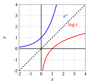
The function \(f: \mathbb{R} \rightarrow \mathbb{R}, x \mapsto e^x\) is strictly increasing on all of \(\mathbb{R}\) and hence invertible; the equation
gives for \(f^{-1}\) the analytic expression
that is, the function: \(f^{-1}: (0,+\infty) \rightarrow \mathbb{R}, y \mapsto \log{y}\).
The graphs \(y=e^x\) and \(y=\log {x}\) are symmetric with respect to the bisector \(y = x\)
-
Now consider the function:
\[ f(x)= x + e^x \]Being the sum of two functions that are strictly increasing on all of \(\mathbb{R}\), \(f(x)\) is strictly increasing and hence invertible on all of \(\mathbb{R}\) (see Theorem Theorem 1). However, we would try in vain to solve the equation \(x + e^x = y\) for \(x\). In other words, \(f^{-1}\) exists, but we cannot write it explicitly.
1.2 Inverse power functions
Given \(\alpha \in \mathbb{R},\alpha \neq 0\), we have:
If \(\alpha > 0\) we have:
If \(\alpha=\frac{m}{n} \in \Q\), with \(m \in \Z, n \in \N_+\) odd and coprime, we have:
-
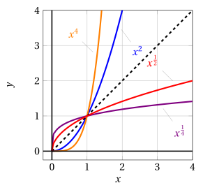
The even powers:
\[ x^{2\:n} {\rm~~~~with~} n = 1, 2, \dots \]are not invertible on the whole real line, but only on the half-line \(x \ge 0\).
-
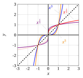
The odd powers:
\[ x^{2\:n+1} {\rm~~~~with~} n = 1, 2, \dots \]and the powers with rational exponent
\[ x^{\frac{m}{n}} {\rm~~with~~} n,m {\rm~~positive ~odd~integers} \]being strictly increasing monotone functions, are invertible from \(-\infty\) to \(+\infty\).
1.3 Inverse trigonometric functions
-
Being periodic, the trigonometric functions cannot be invertible. Indeed, for example, the equation
\[ y = \sin x \]has infinitely many solutions if \(- 1 \le y \le 1\) (the output \(y\) corresponds to infinitely many inputs), or has no real solutions if \(|y| > 1\).
-
To speak of inverse functions of sine, cosine and tangent, we will need to restrict ourselves to intervals on which these functions are strictly monotone and therefore invertible.
-
An interval on which the sine function is invertible is \([-\frac{\pi}{2},\frac{\pi}{2}]\).
Definition 3: of arcsine
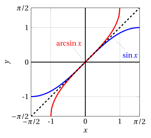
The inverse function of the sine on the interval \(\left[-\frac{\pi}{2},\frac{\pi}{2}\right]\) is the arcsine:
We have:
- The graph of the arcsine is obtained from the arc of the sine curve restricted to the interval \(\left[-\frac{\pi}{2},\frac{\pi}{2}\right]\) (strictly monotone), by symmetry with respect to the bisector \(y = x\),
- An interval on which the cosine function is invertible is \([0,\pi]\).
Definition 4: of arccosine
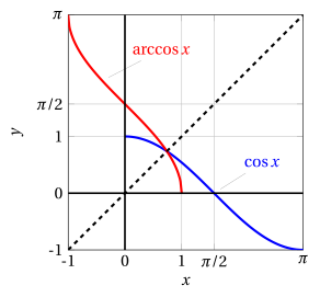
The inverse function of the cosine on the interval \([0,\pi]\) is the arccosine:
We have:
- The graph of the arccosine is obtained from the arc of the cosine curve restricted to the interval \([0,\pi]\) (strictly monotone), by symmetry with respect to the bisector \(y = x\),
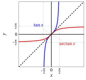
- Note that on the interval \(( -\frac{\pi}{2}, \frac{\pi}{2})\) the tangent is strictly monotone and hence invertible. Its inverse function is called the arctangent (\(\arctan\)), and it is defined on \(\mathbb{R}\).
Definition 5: of arctangent
The inverse function of the tangent on the interval \(\left(-\frac{\pi}{2},\frac{\pi}{2}\right)\) is the arctangent:
We have:
- The graph of the arctangent is obtained from that of the tangent restricted to the interval \(\left(-\frac{\pi}{2},\frac{\pi}{2}\right)\) (strictly monotone), by symmetry with respect to the bisector \(y = x\),
- By means of the inverse trigonometric functions, we can express the solutions of a trigonometric equation or inequality when it involves angles that are not standard angles.
Example 7: Trigonometric equations/inequalities
-
The solutions of:
\[ \sin x = \frac{1}{4} \]are:
\[ (i) ~~~~~~ x = \arcsin \frac{1}{4} + 2\: k \: \pi; ~~~~~~(ii) ~~~~~~ x = \pi - \arcsin \frac{1}{4} + 2\: k \: \pi \qquad (k \in \mathbb{Z}) \]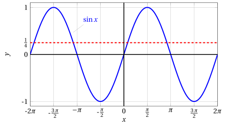
-
The solutions of:
\[ \cos x < \frac{1}{5} \]are:
\[ \arccos \frac{1}{5} + 2\: k \: \pi ~~<~~ x ~~<~~ 2 \: \pi - \arccos \frac{1}{5} + 2\: k \: \pi \qquad (k \in \mathbb{Z}) \]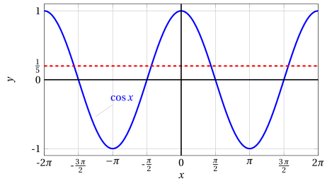
-
The solutions of:
\[ \tan x \ge 3 \]are:
\[ \arctan \:3 + k \: \pi ~~\le~~ x ~~<~~ \frac{\pi}{2} + k \: \pi \qquad (k \in \mathbb{Z}) \]
1.4 Inverse hyperbolic functions
-
Consider the hyperbolic sine function:
\[ y =\sinH x = \frac{e^x - e^{-x}}{2} \]It is defined and strictly increasing on all of \(\mathbb{R}\), therefore it is invertible.
-
To solve the equation for \(x\), multiplying both sides by \(e^x\) we obtain:
\[\begin{align*} 0 & = e^x \: y - e^x \: \frac{e^x - e^{-x}}{2}\\[2ex] & = 2\: e^x \: y - (e^x \: e^x - \underbrace{e^x \: e^{-x}}_{=e^{x-x}=e^0})\\[2ex] & = 2\:y\: e^x - e^{2\:x} + 1 \\[2ex] & = e^{2\:x} - 2\: y \:e^x -1 \end{align*}\]which is a quadratic equation in the unknown \(e^x\). Setting \(t=e^x\) we obtain
\[ 0 = t^{2} - 2\: y \: t -1 \]We obtain:
\[ t = y \pm \sqrt{y^2+1} {\rm~~~~~and~substituting~back~~~~~} e^x = y \pm \sqrt{y^2+1} \]since \(e^x > 0\), the solution with the minus sign must be discarded. Hence we are left with:
\[ e^x = \underbrace{y + \sqrt{y^2+1}}_{>0, \forall y \in \R} {\rm~~~~and~hence~~~~} x = \log \left(y + \sqrt{y^2+1}\right) \] -
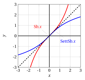
This is the analytic expression of the inverse function of \(\sinH x\), which is called the inverse hyperbolic sine (area hyperbolic sine), and is also denoted by \(\setsinH\). It is defined for every real \(y\).
Definition 6: of inverse hyperbolic sine
The inverse function of the hyperbolic sine is the inverse hyperbolic sine:
We have:
- The graph of the inverse hyperbolic sine is obtained from that of the hyperbolic sine on \(\mathbb{R}\) (strictly monotone), by symmetry with respect to the bisector \(y = x\)
-
Consider the hyperbolic cosine function:
\[ y =\cosH x = \frac{e^x + e^{-x}}{2} \]It is defined on all of \(\mathbb{R}\), strictly increasing for \(x \ge 0\), decreasing for \(x \le 0\). Therefore it is not invertible on all of \(\mathbb{R}\).
-
Its restriction to \(x \ge 0\), however, is invertible. We want to determine the analytic expression of the inverse function of this restriction.
-
Proceeding as before, we obtain:
\[ e^x = y \pm \sqrt{y^2-1} \] -
This time both numbers \(y \pm \sqrt{y^2-1}\) are positive; recall, however, that we are reasoning only for \(x \ge 0\), which is equivalent to choosing the plus sign. Therefore:
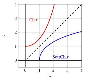
\[ x = \log \left(y + \sqrt{y^2-1}\right) \]This is the analytic expression of the inverse function of \(\cosH x\), which is called the inverse hyperbolic cosine (area hyperbolic cosine), and is also denoted by \(\setcosH\). Note that it is defined for \(y \ge 1\).
Definition 7: of inverse hyperbolic cosine
The inverse function of the hyperbolic cosine on the interval \([0,+\infty)\) is the inverse hyperbolic cosine:
We have:
- The graph of the inverse hyperbolic cosine is obtained from that of the hyperbolic cosine on \([0,+\infty)\) (strictly monotone), by symmetry with respect to the bisector \(y = x\).
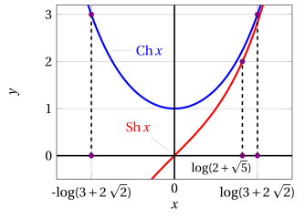
Example 8: Hyperbolic equations
-
The equation:
\[ \sinH x = 2 \]has the unique solution:
\[ x = \setsinH 2 = \log (2 + \sqrt{5}) \] -
The equation:
\[ \cosH x = 3 \]has two solutions:
\[ x = \pm \setcosH 3 = \pm \log(3 + 2\:\sqrt{2}) \]