Power functions

Part 2 · Functions · Chapter 3 · lecture notes by Fabio Furini · Chapter PDF

1. Power functions

Definition 1: power functions

Given \(\alpha \in \R, \alpha \neq 0\), the function:

\[\begin{equation} \label{potenze} f:D \subseteq \R \rightarrow \mathbb{R},~~~ f:x \mapsto x^{\alpha} \end{equation}\]

is called the power function with exponent \(\alpha\). The domain \(D\) depends on the value of \(\alpha\):

• with rational exponent \(\alpha=\frac{m}{n} \in \Q\), \(m \in \Z\) and \(n \in \N_+\) coprime, we have four cases:

  \[ D= \begin{cases} \R & {\rm ~~if~~} n {\rm ~~odd~~} {\rm ~~and~~~} \frac{m}{n}>0\\[2ex] \R \setminus \{0\} & {\rm ~~if~~} n {\rm ~~odd~~} {\rm ~~and~~~} \frac{m}{n}<0\\[2ex] [0,\ip) & {\rm ~~if~~} n {\rm ~~even~~} {\rm ~~and~~~} \frac{m}{n}>0\\[2ex] (0,\ip) & {\rm ~~if~~} n {\rm ~~even~~} {\rm ~~and~~~} \frac{m}{n}<0 \end{cases} \]

• with real, non-rational exponent \(\alpha \in \R \setminus \Q\), we have two cases:

  \[ D= \begin{cases} [0,\ip) & {\rm ~~if~~} \alpha >0\\[2ex] (0,\ip) & {\rm ~~if~~} \alpha<0 \end{cases} \]

1.1 Rational exponent

With \(\alpha=\frac{m}{n} \in \Q\), \(m \in \Z\) and \(n \in \N_+\) coprime, we have a power function with rational exponent:

\[ f:D \subseteq \R \rightarrow \mathbb{R},~~~ f:x \mapsto x^{\frac{m}{n}}=\sqrt[n]{x^m} \]

We have the following three cases, depending on whether \(m\) and \(n\) are even or odd.

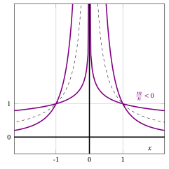
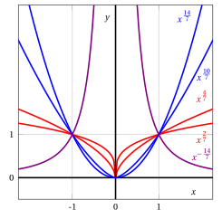
1. With \(n\) odd and \(m\) even, it is an even function, i.e., \((-x)^{\frac{m}{n}}=x^{\frac{m}{n}}\). For the sign and the monotonicity we have:

   \[ x^{\frac{m}{n}} > 0, ~~~\forall x \in \R \setminus \{0\};\qquad x^{\frac{m}{n}} = 0 \Longleftrightarrow x=0 {\rm ~~and~~} \frac{m}{n}>0 \]
   \[ \begin{cases} {\rm ~~if~~} \frac{m}{n} >0 {\rm ~~~then~} f {\rm ~~is~decreasing~in~} (\im,0] {\rm ~~and~increasing~in~} [0,\ip)\\[3ex] {\rm ~~if~~} \frac{m}{n}<0 {\rm ~~~then~} f {\rm ~~is~increasing~in~} (\im,0) {\rm ~~and~decreasing~in~} (0,\ip) \end{cases} \]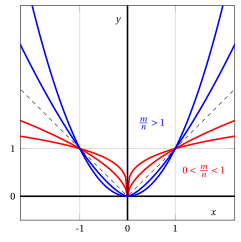

   

   

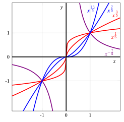
2. With \(n\) odd and \(m\) odd, it is an odd function, i.e., \((-x)^{\frac{m}{n}}=-x^{\frac{m}{n}}\). For the sign and the monotonicity we have:

   \[ x^{\frac{m}{n}} < 0, ~ \forall x < 0,~~~~x^{\frac{m}{n}} > 0, ~ \forall x > 0;\qquad x^{\frac{m}{n}} = 0 \Longleftrightarrow x=0 {\rm ~~and~~} \frac{m}{n}>0 \]
   \[ \begin{cases} {\rm ~~if~~} \frac{m}{n} >0 {\rm ~~~then~} f {\rm ~~is~increasing~in~} \R\\[3ex] {\rm ~~if~~} \frac{m}{n}<0 {\rm ~~~then~} f {\rm ~~is~decreasing~in~} (\im,0) {\rm ~~and~in~} (0,\ip) \end{cases} \]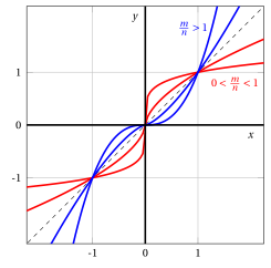

   

   

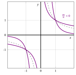
   Example 1: graphs of power functions with rational exponent \(\frac{m}{n}\) and \(n\) odd

   With \(m\) even:

   

   With \(m\) odd:

   

3. With \(n\) even and \(m\) odd (\(m\) cannot be even since they are coprime), for the sign and the monotonicity we have:

   \[ x^{\frac{m}{n}} > 0, ~~~\forall x >0;\qquad x^{\frac{m}{n}} = 0 \Longleftrightarrow x=0 {\rm ~~and~~} \frac{m}{n}>0 \]
   \[ \begin{cases} {\rm ~~if~~} \frac{m}{n} >0 {\rm ~~~then~} f {\rm ~~is~increasing~in~} [0,\ip)\\[3ex] {\rm ~~if~~} \frac{m}{n}<0 {\rm ~~~then~} f {\rm ~~is~decreasing~in~} (0,\ip) \end{cases} \]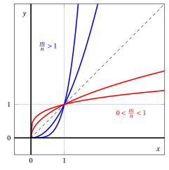

   

   

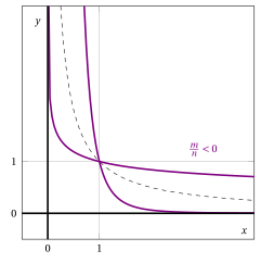
   Example 2: graphs of power functions with rational exponent \(\frac{m}{n}\) and \(n\) even

   

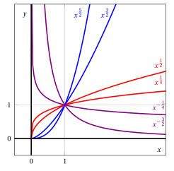
1.2 Real exponent

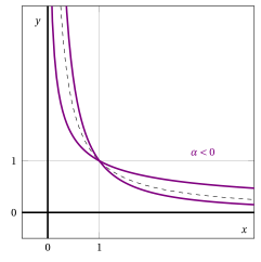
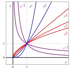
• With \(\alpha \in \R\setminus \Q\), for the sign and the monotonicity we have:

  \[ x^{\alpha} > 0, ~~~\forall x >0;\qquad x^{\alpha} = 0 \Longleftrightarrow x=0 {\rm ~~and~~} \alpha>0 \]
  \[ \begin{cases} {\rm ~~if~~} \alpha >0 {\rm ~~~then~} f {\rm ~~is~increasing~in~} [0,\ip)\\[2ex] {\rm ~~if~~} \alpha<0 {\rm ~~~then~} f {\rm ~~is~decreasing~in~} (0,\ip) \end{cases} \]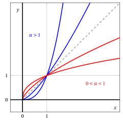

  

  

Example 3: graphs of power functions with real exponent

Try it — the interactive graph below shows what you have just read: move the sliders.

1.3 Polynomials

Definition 2: polynomial

Given \(n+1\) values \(a_i \in \R\) with \(i \in \{0,1,\dots,n\}\) and \(a_n \neq 0\), the function:

\[\begin{equation} \label{potenze__2} f:\R \rightarrow \mathbb{R},~~~ f:x \mapsto \underbrace{\sum_{i=0}^n a_i \: x^i }_{= P_n(x)} \end{equation}\]

is called a polynomial of degree \(n\).

• For each monomial \(i \in \{0,1,\dots,n\}\):

  1. the value \(a_i\) is the coefficient of the monomial

  2. the power function \(x^i\) with integer exponent \(i\) is the literal part of the monomial

  The value \(a_0\) is the constant term of the polynomial since \(x^0=1.\)

Example 4: polynomial

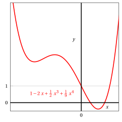
For example, with \(n=4\), \(a_0=1\), \(a_1=-2\), \(a_2=0\), \(a_3=\frac{1}{2}\) and \(a_4=\frac{1}{9}\) we have the following polynomial of degree four:

\[ P_4(x) = \sum_{i=0}^4 a_i \: x^i = 1 - 2 \; x + \frac{1}{2} \; x^3 + \frac{1}{9} \; x^4 \]

2. Direct and inverse proportionality functions

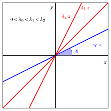
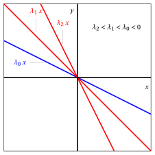
With \(\alpha = 1\) and given \(\lambda \in \mathbb{R}\), we have the family of direct proportionality (or linear) functions:

\[ f:\R \rightarrow \mathbb{R},~~~ f:x \mapsto \lambda \: x {\rm ~~~~where~~} \lambda {\rm ~~is~the~constant~of~direct~proportionality} \]

Moreover, \(\lambda= \tan \vartheta\) and \(\vartheta\) is the angle between the line \(y=\lambda \: x\) and the \(x\)-axis.

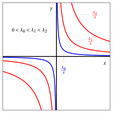
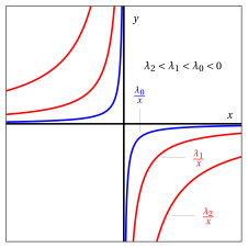
With \(\alpha = -1\) and given \(\lambda \in \mathbb{R}\), we have the family of inverse proportionality functions (or rectangular hyperbolas):

\[ f:\R \setminus \{0\} \rightarrow \mathbb{R},~~~ f:x \mapsto \frac{\lambda}{x} {\rm ~~~~where~~} \lambda {\rm ~~is~the~constant~of~inverse~proportionality} \]

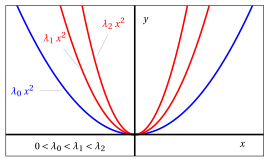
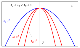
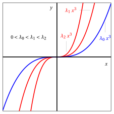
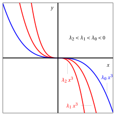
Given \(\alpha \in \R\) and \(\lambda \in \mathbb{R}\), we have the family of power functions multiplied by a constant:

\[ f:D \subseteq \R \rightarrow \mathbb{R},~~~ f:x \mapsto \lambda \: x^{\alpha} {\rm ~~~~where~~} \lambda {\rm ~~is~the~multiplicative~constant} \]

• For example, with \(\alpha\) equal to \(2\) or equal to \(3\) and \(\lambda \in \R\) we have:

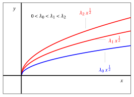
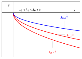
• For example, with \(\alpha=\frac{1}{2}\) and \(\lambda \in \R\) we have: