Fundamental limits and asymptotic estimates
Part 3 · Limits of functions and continuity · Chapter 6 · lecture notes by Fabio Furini · Chapter PDF
1. Fundamental limits
- We now look at some common techniques for computing limits that combine the general theorems on limits with the use of some fundamental limits of certain elementary functions.
1.1 Fundamental limits of sine and cosine
-
We want to compute
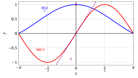
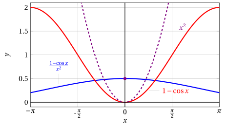
\[ \lim_{x \rr 0} \frac{\sin x}{x} = \left[\frac{0}{0}\right] {\rm ~~and~~} \lim_{x \rr 0} \frac{1-\cos x}{x^2} = \left[\frac{0}{0}\right] \]which are indeterminate forms.
Lemma 1
Proof
The functions \(\sin x\) and \(x\) are odd functions, hence \(\frac{\sin x}{x}\) is an even function. Therefore it is sufficient to compute
We have:
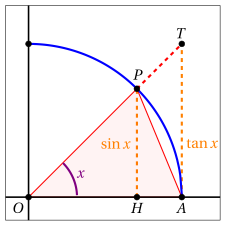
The area of the triangle \(OPA\) is smaller than that of the circular sector \(OPA\), which in turn is smaller than that of the triangle \(OTA\). It follows that
that is, for \(x \in \left(0, \frac{\pi}{2}\right)\):
Dividing by \(\sin x\), which is positive because \(x \in \left(0, \frac{\pi}{2}\right)\), we have
By the comparison theorem, since \(\lim_{x \rr 0} \cos x= 1\), the lemma follows. □
Lemma 2
Proof
We consider
hence, since \(\frac{\sin x}{x} \rr 1 {\rm ~~and~~} (1 + \cos x) \rr 2 {\rm ~~as~~} x \rr 0\), the claim follows. □
1.2 Continuous extension of a function
-
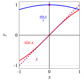
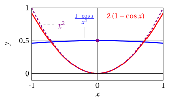
Based on the limit \(\eqref{LN_1}\) just proved, the functions \(f(x) = \frac{\sin x}{x}\) and \(g(x) = \frac{1-\cos x}{x^2}\), initially not defined at \(x = 0\), can be extended by continuity also at \(x = 0\), by setting
\[ f(x)= \begin{cases} \frac{\sin x}{x} & {\rm if~~} x \neq 0\\ 1 & {\rm if~~} x = 0 \end{cases} \qquad g(x)= \begin{cases} \frac{1- \cos x}{x^2} & {\rm if~~} x \neq 0\\ \frac{1}{2} & {\rm if~~} x = 0 \end{cases} \]The functions \(f\) and \(g\) defined in this way are continuous also at \(x = 0\).
-
if a function \(f(x)\) is not defined at \(x_0\) but the finite limit exists
\[ \lim_{x \rr x_0} f(x) = \ell \]the function can be extended by continuity also at \(x_0\), by defining
\[ f(x_0) = \ell \] -
If instead the function \(f\) has at \(x_0\) a jump discontinuity, a vertical asymptote, or in any case does not have a finite limit, it is not possible to make it continuous at \(x_0\) by changing its definition at a single point.
1.3 Other fundamental limits
-
We know that for every sequence \(\{a_n\}\) diverging to \(\ip\) or \(\im\) we have
\[ \lim_{n \rr \ip} \left(1 + \frac{1}{a_n}\right)^{a_n} = e \] -
By the sequential definition of the limit of a function, this fact immediately implies the next fundamental limit
Lemma 3
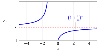
If \(\eta(x)\) is a function that tends to infinity1 (i.e., it is an infinity: \(\eta(x) \rr \pm\infty\)), we have:
Example 1: Limits of functions tending to \(e\)
1.
$$
\lim_{x \rr \ip} \left( 1 + \frac{1}{2\:x^2-10} \right)^{2\:x^2-10} = e
$$

since with $\eta(x) = 2\:x^2-10$ we have

$$
\eta(x) \rr \ip {\rm~~as~~} x \rr \ip.
$$
2.
$$
\lim_{x \rr 0^+} \left( 1 + \frac{1}{1/x} \right)^{1/x} = e
$$

since with $\eta(x) = \frac{1}{x}$ we have

$$
\eta(x) \rr \ip {\rm~~as~~} x \rr 0^+.
$$
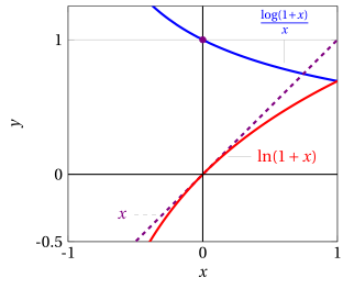
From the fundamental limit \(\eqref{LN_3}\) three more can be deduced
Corollary 1
Proof
Taking logarithms in \(\eqref{LN_3}\), we obtain
hence
Now, if we set \(y=\frac{1}{x}\), \(x \rr \pm \infty\) is equivalent to \(y \rr 0^{\pm}\), and the last limit can therefore be rewritten in the following form:
□
Corollary 2
Proof
If in \(\eqref{LN_4}\) we instead set \(y= e^x -1\), \(y \rr 0\) is equivalent to \(x \rr 0\), and substituting we obtain
Taking reciprocals we obtain the fundamental limit. □
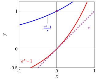
Example 2: Fundamental limit
We compute:
We set \(z= -x\); \(x \rr 0\) is equivalent to \(z \rr 0\), and substituting we obtain:
Corollary 3
Proof
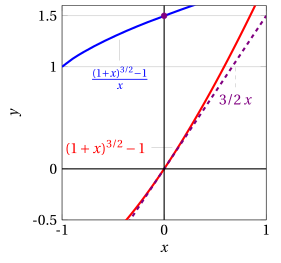
If in \(\eqref{LN_4}\) we instead set \(y= (1+x)^{\alpha} -1\), with \(\alpha\) any real exponent, then \(x \rr 0\) is equivalent to \(y \rr 0\) and we have:
But since also
then
Taking reciprocals and then multiplying by \(\alpha\) we obtain the fundamental limit. □
2. Asymptotic estimates
Definition 1: Asymptotic functions
Two functions \(f\) , \(g\) are said to be asymptotic as \(x \rr c\) if
and we write \(f \thicksim g\) as \(x \rr c\).
- The asymptotic symbol for functions enjoys all the properties stated for sequences
As \(x \rr 0\) we have (from the fundamental limits):
- The functions \(\thicksim x\) behave, to a first approximation or to first order, like \(x\) as \(x \rr 0\).
If \(\varepsilon(x)\) is a function that tends to zero2 (i.e., it is an infinitesimal: \(\varepsilon(x) \rr 0\)), we have:
-
Formulas \(\eqref{LIM_NOT_C__2}\) follow from formulas \(\eqref{LIMMMM}\) simply by a change of variable
\[ x = \varepsilon(x) \]
Example 3: Limits with asymptotic functions
We use the estimate
with
Then, as \(x \rr 1\), we have
and
Example 4: Limits with asymptotic functions
We use the estimate
with
Hence, as \(x \rr 0\) we have
Now we also use the estimate
with
Hence, as \(x \rr 0\) we have
Then, as \(x \rr 0\), we have
and
Example 5: Limits with asymptotic functions
We rewrite,
We use the estimate
with
Then, as \(x \rr \ip\), we have
and
3. Asymptotic estimates and graphs
- Asymptotic estimates are useful not only for computing limits, but also for sketching the qualitative graph of a function in a neighborhood of a given point, or as \(x \rr \pm \infty\).
Example 6: Known graphs
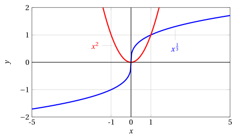
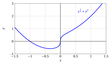
Example 7: Qualitative graph
We now want to study the qualitative graph of the function (the sum of the previous two):
-
the function is defined and continuous on all of \(\R\);
-
as \(x \rr \pm \infty\), \(f(x) \thicksim x^2\), since
\[ \lim_{x \rr \pm \infty} \frac{x^{\frac{1}{3}} + x^2}{x^2} =1 \]Therefore \(f(x) \rr \ip\) as \(x \rr \pm \infty\); moreover, for \(x\) large in absolute value, its graph will be similar to that of \(x^2\).
-
Moreover, the function vanishes at \(x = 0\) and, as \(x \rr 0\), \(f(x) \thicksim x^{\frac{1}{3}}\), since
\[ \lim_{x \rr 0} \frac{x^{\frac{1}{3}} + x^2}{x^{\frac{1}{3}}} =1 \]therefore, in a neighborhood of \(x = 0\), its graph will be similar to that of \(x^{\frac{1}{3}}\); in particular, it will have a vertical tangent at the origin.
Example 8: Actual graph
-
Often the behavior of a function in a neighborhood of a point (for example, the fact that it has a vertical or horizontal tangent) can be predicted from a suitable asymptotic estimate.
-
The asymptotic estimate allows us to sketch the qualitative graph of \(f\) (in a neighborhood of the point) by comparison with that of a known function (for example, a power with rational exponent).
-
Analogous estimates are useful as \(x \rr \pm \infty\).
Growth of a function at infinity
-
Suppose we want to sketch the graph of a function \(f\) that, as \(x \rr \ip\) (or \(\im\)), tends to \(\ip\) (or \(\im\)).
-
To describe the speed at which the function tends to infinity, the following notions are useful: we say that, as \(x \rr \ip\),
\[ f {\rm~~has} \begin{cases} {\rm superlinear~growth}\\ {\rm linear~growth}\\ {\rm sublinear~growth}\\ \end{cases} \quad {\rm if} \quad \lim_{x \rr \ip} \frac{f(x)}{x}= \begin{cases} \pm \infty\\ m ~~~~({\rm ~finite~and~different~from~} 0)\\ 0\\ \end{cases} \] -
Analogous definitions are given for \(x \rr \im\).
-
Only when a function has linear growth is it possible for it to have an oblique asymptote
Example 9: Growth of a function at infinity
For example, as \(x \rr \ip\)
-
Superlinear growth:\(~~~\) exponentials \(a^x\) and powers \(x^a\) with \(a > 1\).
-
Sublinear growth:\(~~~\) logarithms \(\log_a x\) and powers \(x^a\) with \(0 < a < 1\).
Example 10: Growth of a function at infinity
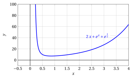
The function
-
as \(x \rr \ip\) it is asymptotic to \(e^x\); therefore it tends to \(\ip\) with superlinear growth;
-
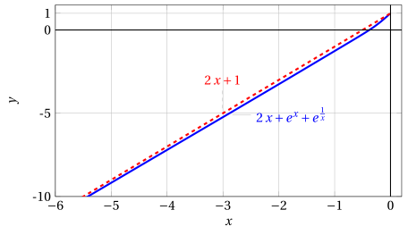
as \(x \rr \im\) it is asymptotic to \(2\:x\); therefore it tends to \(\im\) linearly
-
since
\[ \lim_{x \rr \im}[f(x) - 2\:x] = 1 \]the function has the oblique asymptote
\[ y = 2\:x + 1 {\rm ~~as~~} x \rr \im \]
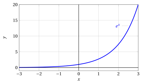
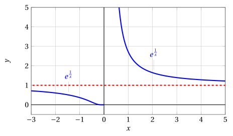
Example 11: Graphs
Example 12: Actual graph