Operations on graphs
Part 2 · Functions · Chapter 9 · lecture notes by Fabio Furini · Chapter PDF
1. Operations on graphs
- Knowing the graph of a function \(y = f (x)\), by means of simple geometric transformations it is possible to draw the graph of the following functions:
- Therefore, starting from the elementary functions, it is possible to build, by means of these operations, a large variety of new functions. These operations create translations, dilations and reflections of the original function.
1.1 Operations related to \(y_1= f(x) +a\)
Example 1: Operations on graphs related to \(y_1= f(x) +a\)
Consider \(y = \ln x\). Then
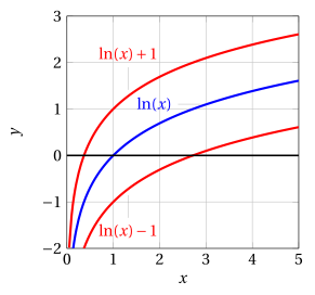
- The graph of \(y_1\) is obtained from that of \(y\) by a translation of \(a\) units upward if \(a> 0\), downward if \(a < 0\).
1.2 Operations related to \(y_2= f(x +a)\)
Example 2: Operations on graphs related to \(y_2= f(x +a)\)
Consider again \(y = \ln x\). Then
Since \(\ln x\) is defined for \(x > 0\), \(\ln(x +a)\) will be defined for \(x +a > 0\), i.e., for \(x > - a\). Since \(\ln x =0\) if \(x = 1\), we have \(\ln(x +a) =0\) for \(x +a= 1\), i.e., \(x = 1 - a\).
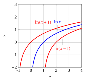
- The graph of \(y_2\) is obtained from that of \(y\) by a translation of \(a\) units to the left if \(a > 0\), to the right if \(a < 0\).
1.3 Operations related to \(y_3 = k\: f(x)\)
-
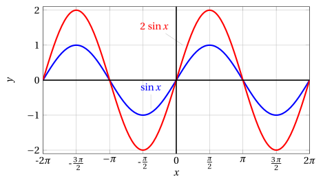
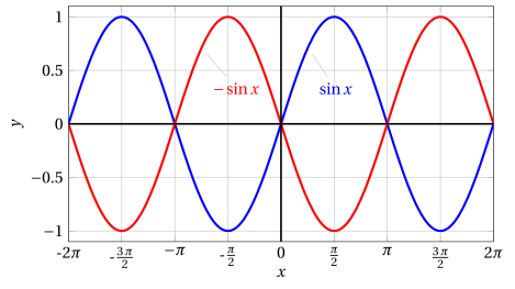
The graph of \(y_3 = k \: f ( x)\) is obtained from that of \(f\) by multiplying all the ordinates \(f(x)\) by \(k\).
-
In particular, if \(k = -1\) the ordinates simply change sign, so that the graph of \(y_3\) is symmetric to that of \(f\) with respect to the \(x\)-axis.
-
Note that if \(k > 1\), the graph is “stretched” in the vertical direction, dilating the positive ordinates upward and the negative ones downward.
-
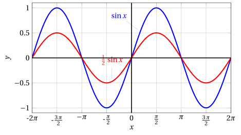
Conversely, if \(0 < k < 1\) the graph “shrinks”, again in the vertical direction.
-
Therefore, the operation of multiplying \(f ( x)\) by \(k\) has the geometric meaning of a dilation (if \(|k| > 1\)) or a contraction (if \(|k| < 1\)) along the \(y\)-axis, possibly accompanied by a reflection with respect to the \(x\)-axis, if \(k < 0\).
Example 3: Operations on graphs related to \(y_3= k\: f( x)\)
Consider \(y = \sin x\), then \(y_3 = k\: \sin(x).\)
1.4 Operations related to \(y_4= f(k\:x)\)
-
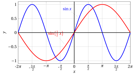
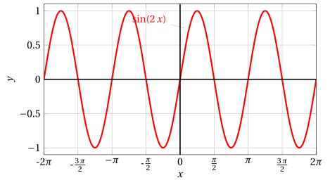
The graph of \(y_4 = f ( k\:x)\) is obtained from that of \(f(x)\) by a change of scale along the \(x\)-axis.
-
If \(k > 1\), \(k \:x\) grows faster than \(x\), and therefore the graph of \(y_4\) will be similar to that of \(f\) but with faster oscillations, that is, it will be “compressed” in the horizontal direction by a factor \(\frac{1}{k}\).
-
Similarly, if \(0 < k < 1\) the graph will appear “dilated” in the horizontal direction, with gentler oscillations.
-
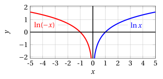
If \(k < 0\), in addition to a compression (if \(|k| > 1\)) or a dilation (if \(|k|< 1\)) along the \(x\)-axis, there will be a reflection with respect to the \(y\)-axis.
Example 4: Operations on graphs related to \(y_4 = f(k\: x)\)
Consider \(y = \sin x\), then \(y_4 = \sin(k\: x).\) With \(k=\frac{1}{2}\) and \(k=2\) we have:
Example 5: Operations on graphs related to \(y_4= f(k\: x)\)
Consider \(y = \ln x\), then \(y_4 = \ln(k\: x).\) With \(k=-1\) we have:
1.5 Operations related to \(y_5=|f(x)|\)
Absolute value of \(f(x)\):
-
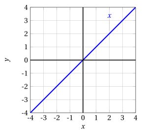
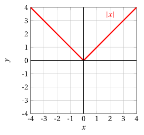
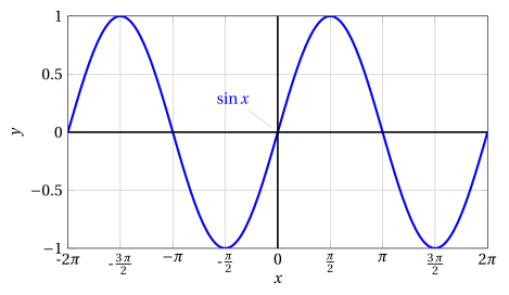
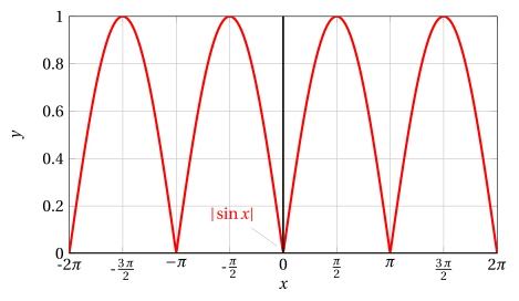
When passing from the graph of \(y=f(x)\) to that of \(y_5=|f(x)|\), the points with non-negative ordinate remain unchanged, while those with negative ordinate are transformed into their symmetric points with respect to the \(x\)-axis.
-
The graph of \(y_5=|f(x)|\) is obtained from that of \(f\) by “flipping” symmetrically with respect to the \(x\)-axis the part of the graph of \(f\) that lies in the lower half-plane, and leaving the rest unchanged.
Example 6: Operations on graphs related to \(y_5= |f(x)|\)
Consider \(y = x\), then \(y_5 = |x|\)
Example 7: Operations on graphs related to \(y_5= |f( x)|\)
Consider \(y = \sin x\), then \(y_5 = |\sin x|\)
1.6 Operations related to \(y_6=f(|x|)\)
-
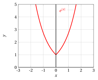
Finally, to draw the graph of \(y_6 =f(|x|)\), we observe that \(|x| = x\) for \(x \ge 0\), and hence in the right half-plane the two graphs coincide.
-
We have \(|-x|=|x|\), and hence \(y_6\) is an even function, therefore symmetric with respect to the \(y\)-axis.
-
Consequently, the graph of \(y_6 = f(|x|)\) is drawn by leaving the graph of \(f\) unchanged in the right half-plane and flipping it symmetrically with respect to the \(y\)-axis.
Example 8: Operations on graphs related to \(y_6=f(|x|)\)
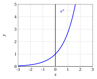
Consider \(y = e^x\), then \(y_6 = e^{|x|}\)
Try it — the interactive graph below shows what you have just read: move the sliders.