Mean value theorem, maxima and minima¶

Part 4 · Derivatives · Chapter 5 · lecture notes by Fabio Furini · Chapter PDF

1. Local and global maxima/minima¶

One of the uses of differential calculus is the search for maxima and minima, that is, the optimization of a function defined on an interval \(I\) (closed/open, bounded/unbounded).

Definition 1: of maximum point and maximum

Given a function \(f:I \rr \R\), if there exists a point \(\tilde{x}_M \in I\) such that:

\[ f(\tilde{x}_M) \ge f(x),~~~ \forall x \in I \]

then \(\tilde{x}_M\) is a (global) maximum point and \(f(\tilde{x}_M)\) is the (global) maximum of \(f\) in \(I\).

Definition 2: of minimum point and minimum

Given a function \(f:I \rr \R\), if there exists a point \(\tilde{x}_m \in I\) such that:

\[ f(\tilde{x}_m) \le f(x),~~~ \forall x \in I \]

then \(\tilde{x}_m\) is a (global) minimum point and \(f(\tilde{x}_m)\) is the (global) minimum of \(f\) in \(I\).

We call an extremum a maximum or a minimum, and an extremum point a maximum or minimum point. An extremum, if it exists, is unique, while there may be several extremum points (even infinitely many).

Definition 3: of local maximum point and local maximum

Given a function \(f:I \rr \R\), if there exist a point \(\bar{x}_M \in I\) and a neighborhood \((\bar{x}_M-\delta,\bar{x}_M+\delta)\) with \(\delta >0\), such that:

\[ f(\bar{x}_M) \ge f(x),~~~ \forall x \in (\bar{x}_M-\delta,\bar{x}_M+\delta) \cap I \]

then \(\bar{x}_M\) is a local maximum point and \(f(\bar{x}_M)\) is the local maximum of \(f\) in \((\bar{x}_M-\delta,\bar{x}_M+\delta) \cap I\).

Definition 4: of local minimum point and local minimum

Given a function \(f:I \rr \R\), if there exist a point \(\bar{x}_m \in I\) and a neighborhood \((\bar{x}_m-\delta,\bar{x}_m+\delta)\) with \(\delta >0\), such that:

\[ f(\bar{x}_m) \le f(x),~~~ \forall x \in (\bar{x}_m-\delta,\bar{x}_m+\delta) \cap I \]

then \(\bar{x}_m\) is a local minimum point and \(f(\bar{x}_m)\) is the local minimum of \(f\) in \((\bar{x}_m-\delta,\bar{x}_m+\delta) \cap I\).

Global extremum points are also local extremum points, and global extrema are also local extrema.

Example 1: extrema and extremum points (global and local)

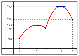
Consider the function \(f\) with the following graph:

the global maximum is \(f (x_2)\) and \(x_2\) is a global maximum point (it is also unique); \(f(x_0)\) is a local (not global) maximum and \(x_0\) is a local (not global) maximum point
the global minimum is \(f (a)\) and \(a\) is a global minimum point (it is also unique); \(f(b)\) and \(f(x_1)\) are two local (not global) minima and \(b\) and \(x_1\) are two local (not global) minimum points

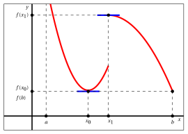
Now consider the function \(f\) with the following graph:

the global maximum does not exist (\(\lim_{x \to a^+} f(x)=\ip\)); \(f(x_1)\) is a local (not global) maximum and \(x_1\) is a local (not global) maximum point
the global minimum is \(f(x_0)\), which is also equal to \(f(b)\); \(x_0\) and \(b\) are two global minimum points

2. Fermat's theorem and stationary points¶

At a local or global extremum point the function may fail to be differentiable and may even be discontinuous. However, the following theorem tells us that if a function is differentiable at a local extremum point, then at that point the derivative vanishes and hence the tangent to the graph is horizontal.

Theorem 1: Fermat's theorem

Given a function \(f: (a,b) \rr \R\) differentiable at \(x_0 \in (a,b)\), if \(f\) has a local extremum at \(x_0\) then \(f'(x_0) = 0\).

Proof

Consider the case where \(x_0\) is a local maximum point. Then:

\[ \exists (x_0-\delta,x_0+\delta) {\rm ~~with~~} \delta >0:~~~ f(x_0) \ge f(x) , ~~\forall x \in (x_0-\delta,x_0+\delta) \cap (a,b) \]

Therefore for every \(x \in (x_0-\delta,x_0+\delta) \cap (a,b)\) we have:

\[ x < x_0 \Rightarrow \frac{f(x)-f(x_0)}{x-x_0} \ge 0 {\rm ~~~~and~hence~~~~} f'_{-}(x_0)=\lim_{x\rr x_0^-} \frac{f(x)-f(x_0)}{x-x_0} \ge 0 \]

where for the non-negativity of the limit we used the sign-preservation theorem. On the other hand:

\[ x > x_0 \Rightarrow \frac{f(x)-f(x_0)}{x-x_0} \le 0 {\rm ~~~~and~hence~~~~} f'_{+}(x_0)=\lim_{x\rr x_0^+} \frac{f(x)-f(x_0)}{x-x_0} \le 0 \]

Since \(f\) is differentiable at \(x_0\), we have:

\[ f'(x_0) = f'_{-}(x_0) = f'_{+}(x_0) =0 \]

The case where \(x_0\) is a local minimum point is handled in the same way. □

Proof

Suppose, by contradiction, that \(f'(x_0) > 0\); then by the sign-preservation theorem we would have \(\frac{f(x) -f(x_0)}{x - x_0} >0\) eventually as \(x \rr x_0\). Taking into account the sign of \(x - x_0\), this implies that \(f(x) > f(x_0)\) eventually as \(x \rr x_0^+\) and \(f(x) < f(x_0)\) eventually as \(x \rr x_0^-\). But this contradicts the hypothesis that \(x_0\) is a local extremum point of \(f\). Similarly, we rule out the case \(f'(x_0) < 0\). Therefore we must have \(f'(x_0) = 0\). □

Definition 5: stationary point

A point \(x_0\) is called a stationary point of \(f\) if \(f\) is differentiable at \(x_0\) and \(f'(x_0) = 0\).

Fermat's theorem says that for a function \(f: (a, b) \rr \R\) differentiable at \(x_0 \in (a,b)\) we have:

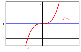
\[\begin{equation} x_0 {\rm ~~is~a~local~extremum~point} ~~~\Rightarrow~~~ \underbrace{x_0 {\rm ~~is~a~stationary~point}}_{ f'(x_0)=0} \label{BBB} \end{equation}\]

Hence “\(x_0\) is a local extremum point” is a sufficient condition for “\(x_0\) is a stationary point”. But the converse is not true. A counterexample is given by the function \(f(x) = x^3+1, \forall x \in \R\), whose derivative function is \(f'(x) = 3\:x^2, \forall x \in \R\). With \(x_0=0\) we have \(f'(0)=0\) but \(x_0= 0\) is not a local extremum point.

Hence we have:

\[ \underbrace{x_0 {\rm ~~is~a~stationary~point}}_{ f'(x_0)=0} ~~~\nRightarrow~~~ x_0 {\rm ~~is~a~local~extremum~point} \]

Finally, from the contrapositive of \(\eqref{BBB}\), we have:

\[ x_0 {\rm ~~is~not~a~stationary~point} ~~\Rightarrow~~ x_0 {\rm ~~is~not~a~local~extremum~point~} \]

3. Mean value theorem (Lagrange's theorem)¶

Theorem 2: mean value theorem (Lagrange)

Given a function \(f\) differentiable in \((a, b)\) and continuous in \([a, b]\), then:

\[\begin{equation} \exists~ c \in (a,b) ~~:~~ \frac{f(b)-f(a)}{b-a}=f'(c) \label{VVV} \end{equation}\]

In the case \(f(b) = f(a)\), the theorem tells us that there exists \(c \in (a,b)\) such that \(f'(c)=0\), that is, there exists at least one point where the derivative vanishes. This corollary of Lagrange's theorem is called Rolle's theorem.

Differentiability is required only on the open interval \((a,b)\) in order to include also functions that are continuous at one of the endpoints but not differentiable there. For example, with \(a=0\):

\[ f(x) = \begin{cases} \sin \left(\frac{1}{x} \right) \; x & {\rm if~~} x \in (0,b)\\ 0 & {\rm if~~} x = 0 \end{cases} ~~~{\rm ~~or~~~} g(x) = \sqrt{x} \]
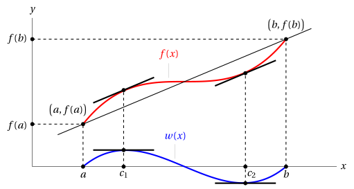
Geometrically, considering the graph of \(f\) we have:
1. \(\frac{f(b)-f(a)}{b-a}\) is the slope of the line through \(\big(a, f(a)\big)\) and \(\big(b,f(b)\big)\)
2. \(f'(c)\) is the slope of the tangent line to the graph of \(f\) at the point \(\big(c,f(c)\big)\)
The mean value theorem therefore expresses the fact that at the point \(\big(c,f(c)\big)\) the tangent to the graph of \(f\) is parallel to the line through \(\big(a, f(a)\big)\) and \(\big(b,f(b)\big)\). There may be more than one point with this property, as the following figure shows:
The figure also shows the function

\[ w(x) = f(x) - \left( f(a) + \frac{f(b)-f(a)}{b-a} \;(x-a) \right) \]

given by the difference between the values of the function and the line through the points \(\big(a, f(a)\big)\) and \(\big(b,f(b)\big)\), which has equation:

\[ y = f(a) + \frac{f(b)-f(a)}{b-a} \; (x-a) \]

The function \(w(x)\) is the key to the proof of the theorem.

Proof

Consider the function:

\[ w(x) = f(x) - \left( f(a) + \frac{f(b)-f(a)}{b-a} \;(x-a) \right) \]

Clearly \(w(a)=w(b)=0\); moreover \(w\) is continuous in \([a,b]\) and differentiable in \((a,b)\). Since

\[ w'(x) = f'(x) - \frac{f(b)-f(a)}{b-a} {\rm ~~~then~~~} \frac{f(b)-f(a)}{b-a}=f'(c) \Longleftrightarrow \exists c\in (a,b): w' (c) = 0 \]

Since \(w\) is continuous in \([a, b]\), by the Weierstrass theorem there exist two points \(x_1\) and \(x_2\) in \([a, b]\) such that:

\[ w(x_1) = M, {\rm ~the~maximum~of~} w {\rm~in~} [a, b];~~~w(x_2) = m, {\rm ~the~minimum~of~} w {\rm~in~} [a, b]. \]

If \(M = m\), then \(w(x)\) is constant in \([a,b]\), and hence \(w'(x) =0, \forall x \in (a,b)\).

If \(M > m\), at least one of the two points \(x_1\) or \(x_2\) is not at the endpoints of the interval, since \(w(a) = w(b) = 0\). Fermat's theorem then implies that at the maximum or minimum point that lies in the interior (possibly both) the derivative of \(w\) vanishes, and the theorem is thus proved. □

Example 2: using the mean value theorem

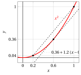
Let \(f(x) = x^2\). Then \(f'(x) = 2\:x\) and the mean value theorem states that in every interval \([a, b]\) there exists a number \(c\) such that:

\[ \frac{b^2-a^2}{b-a}=2\:c {\rm ~~~~from~which~~~~} c= \frac{a+b}{2} \qquad ({\rm arithmetic~mean}) \]

That is, every chord \(AB\) of the parabola \(y = x^2\) is parallel to the tangent at the point whose abscissa equals the arithmetic mean of the abscissas of \(A\) and \(B\). Taking for example the interval \([0.2,1]\) (\(a=0.2,b=1\) and \(c=0.6\)), we have:

Example 3: using the mean value theorem

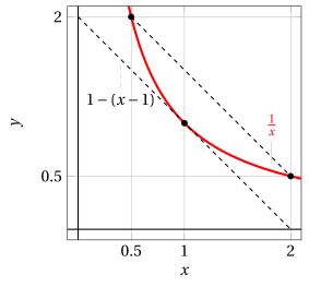
Let \(f(x) = \frac{1}{x}\). Then \(f'(x) = - \frac{1}{x^2}\) and the mean value theorem states that in every interval \([a, b]\) there exists a number \(c\) such that:

\[ \frac{\frac{1}{b}-\frac{1}{a}}{b-a}=- \frac{1}{c^2} {\rm ~~~~from~which~~~~} c= \sqrt{a \cdot b} \qquad ({\rm geometric~mean}) \]

That is, every chord \(AB\) of the hyperbola \(y = \frac{1}{x}\) is parallel to the tangent at the point whose abscissa equals the geometric mean of the abscissas of \(A\) and \(B\). Taking for example the interval \([0.5,2]\) (\(a=0.5,b=2\) and \(c=1\)), we have:

Try it — the interactive graph below shows what you have just read: move the sliders.

4. Differential monotonicity test theorem¶

!!! teorema "Theorem 3: Differential Monotonicity Test"

Given a function $f:I \rr \R$, continuous in $I$ and differentiable at the interior points of $I$, then:

\begin{align}
\label{C1} f'(x) \ge 0,~ \forall x {\rm ~in~the~interior~of~} I &~~~\Longleftrightarrow~~~  f {\rm ~is~non\text{-}decreasing~in~} I\\[2ex]
\label{C2} f'(x) \le 0,~ \forall x {\rm ~in~the~interior~of~} I &~~~\Longleftrightarrow~~~  f {\rm ~is~non\text{-}increasing~in~} I\\[2ex]
\label{C3} f'(x) > 0,~ \forall x {\rm ~in~the~interior~of~} I &~~~\Longrightarrow~~~  f {\rm ~is~increasing~in~} I\\[2ex]
\label{C4} f'(x) < 0,~ \forall x {\rm ~in~the~interior~of~} I &~~~\Longrightarrow~~~  f {\rm ~is~decreasing~in~} I
\end{align}

Proof

(\(\Rightarrow\)) Taking two points \(x_1 < x_2\) in the interval \(I\), we can apply Lagrange's theorem on the interval \([x_1,x_2]\), hence there exists \(c \in (x_1, x_2)\) such that

\[ f(x_2) - f(x_1) = f'(c)(x_2 - x_1) \]

If \(f'(c) \ge 0\) (resp. > 0), then \(f(x_2) \ge f(x_1)\) (resp. \(f(x_2) > f(x_1)\)). Since \(x_1\) and \(x_2\) are arbitrary, we have proved that \(f\) is non-decreasing (resp. increasing) in \(I\). If \(f'(c) \le 0\) (resp. < 0) the argument is analogous.
(\(\Leftarrow\)) If \(f\) is non-decreasing, then we have

\[ \frac{f(z)-f(x)}{z-x} \ge 0 {\rm ~~~for~all~}z,x \in I, z \neq x \]

and, by the sign-preservation theorem, the limit of the ratio as \(z \rr x\) is also non-negative; by hypothesis this limit exists and equals \(f'(x)\) for every \(x\) in the interior of \(I\). If \(f\) is non-increasing the argument is analogous.

□

The Differential Monotonicity Test theorem says that for a function \(f: I \rr \R\) differentiable at the interior points of \(I\) we have:

\[ f'(x) \ge 0,~ \forall x {\rm ~in~the~interior~of~} I ~~~\Longleftrightarrow~~~ f {\rm ~is~non\text{-}decreasing~in~} I \]

Hence “\(f'(x) \ge 0,~ \forall x\) in the interior of \(I\)” is a necessary and sufficient condition for “\(f\) is non-decreasing in \(I\)”. The same holds for the case of non-increasing functions.

The Differential Monotonicity Test theorem says that for a function \(f: I \rr \R\) differentiable at the interior points of \(I\) we have:

\[ f'(x) > 0,~ \forall x {\rm ~in~the~interior~of~} I ~~~\Longrightarrow~~~ f {\rm ~is~increasing~in~} I \]

Hence “\(f'(x) > 0,~ \forall x\) in the interior of \(I\)” is a sufficient condition for “\(f\) is increasing in \(I\)”. But the converse is not true. A counterexample is given by the function \(f(x) = x^3+1, \forall x \in \R\), which is increasing and differentiable in \(\R\), but \(f'(x) = 3\;x^2\) vanishes at \(x_0 = 0\).

Hence we have:

\[ f {\rm ~is~increasing~in~} I ~~~\nRightarrow~~~ f'(x) > 0,~ \forall x {\rm ~in~the~interior~of~} I \]

Finally, from the contrapositive of \(\eqref{C3}\), we have:

\[ f {\rm ~is~not~increasing~in~} I ~~\Rightarrow~~ ~ \exists x {\rm ~in~the~interior~of~} I: f'(x) \le 0, \]

To be checked. The same holds for the case of decreasing functions.

It follows immediately from the theorem that with \(I=(a,b)\) we have:

\[\begin{align*} f'(x) = 0,~ \forall x \in (a, b) &~~~\Longrightarrow~~~ f {\rm ~~constant~in~} (a, b) \end{align*}\]

The converse implication is obvious. We then have

\[\begin{align} \label{C5} f'(x) = 0,~ \forall x \in (a, b) &~~~\Longleftrightarrow~~~ f {\rm ~~constant~in~} (a, b) \end{align}\]

Hence “\(f'(x) = 0,~ \forall x \in (a, b)\)” is a necessary and sufficient condition for “\(f\) constant in \((a,b)\)”.

Example 4: functions with zero derivative

Consider the function:

\[ f(x) = \arctan x + \arctan \frac{1}{x},~~~ \forall x \neq 0 \]

we have

\[ f'(x) = \frac{1}{1+x^2} + \frac{1}{1+\frac{1}{x^2}} \; \left(-\frac{1}{x^2}\right)=0,~~~ \forall x \neq 0 \]

Implication \(\eqref{C5}\) allows us to say that \(f\) is constant on the interval \((-\infty,0)\) and on the interval \((0,\infty)\). To find its value, it is enough to compute \(f\) at one point of each interval, for example:

\[ f(1) = \arctan (1) + \arctan (1) = 2 \; \frac{\pi}{4}=\frac{\pi}{2} \]

\[ f(-1) = \arctan (-1) + \arctan (-1) = -\frac{\pi}{2} \]

We have therefore proved that:

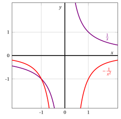
\[ \arctan x + \arctan \frac{1}{x} = \begin{cases} \frac{\pi}{2} & {\rm ~~if~~} x>0\\[2ex] -\frac{\pi}{2} & {\rm ~~if~~} x<0 \end{cases} \]

Both in the Differential Monotonicity Test theorem and in implication \(\eqref{C5}\) it is essential that the set \(I\) is an interval. For example, the function

\[ f(x) = \frac{1}{x},~~ \forall x \in \R \setminus \{0\} \]

has derivative

\[ f'(x) = -\frac{1}{x^2} < 0,~~ \forall x \in \R \setminus \{0\} \]

but the function is not decreasing on its domain. The function is decreasing on the interval \((-\infty,0)\) and on the interval \((0,\infty)\), as the figure shows:

5. Finding maxima and minima¶

Suppose we have a function \(f:[a, b] \rr \R\) and we want to find its local and global maxima and minima in \([a,b]\). If \(f\) is differentiable in \((a,b)\) we can proceed as follows:

Compute \(f(a)\) and \(f(b)\).
Compute \(f'(x)\) and solve the equation \(f'(x)=0\). In this way we find the stationary points, among which are the possible local extremum points in the interval \((a,b)\).
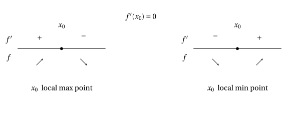
If there are no stationary points, \(f(a)\) and \(f(b)\) are the global extrema and \(a\) and \(b\) are global extremum points. Otherwise we need to determine the nature of the stationary points found. The function \(f\) has a local extremum at a stationary point if and only if the sign of \(f'\) changes there, which we check by studying the sign of \(f'\) in a neighborhood of the point. We have the following cases:

Having found the possible local extremum points, compute the value of \(f\) at these points and compare it with \(f(a)\) and \(f(b)\) to understand whether or not they are global extremum points; in this way the global extrema are determined.

Example 5: finding maxima and minima

Consider the function:

\[ f(x) = x \; e^{-x^2}, {\rm ~~with~~} x \in [0,2] \]

Step 1:

\[ f(0)=0,~~f(2)=2\; e^{-4} \]

Example 6: finding maxima and minima

Step 2:

\[ f'(x) = e^{-x^2} + x \; e^{-x^2} \; (-2\:x) = e^{-x^2} \;(1 - 2\:x^2) \]

We have \(e^{-x^2} > 0, \forall x \in \R\), hence:

\[ f'(x) = 0 \Longleftrightarrow (1 - 2\:x^2)=0 \Longleftrightarrow x=\pm \frac{1}{\sqrt{2}} \]

Only \(\frac{1}{\sqrt{2}} \in [0,2]\), hence we have the stationary point \(x_0 = \frac{1}{\sqrt{2}}\).

Step 3:

We study the sign of \(f'\) near \(x_0 = \frac{1}{\sqrt{2}}\). We have \(f'(x) \ge 0\) for \(2\:x^2 \le 1\), that is, for \(-\frac{1}{\sqrt{2}} \le x \le \frac{1}{\sqrt{2}}\)

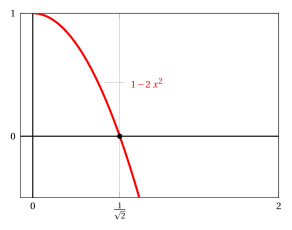
We therefore conclude that:

\[ \frac{1}{\sqrt{2}} {\rm ~~is~a~local~ maximum~point~~~and~~~} f\left(\frac{1}{\sqrt{2}}\right) = \frac{1}{\sqrt{2}} \; e^{-1/2} = \frac{1}{\sqrt{2\: e}} {\rm ~~is ~a~local~maximum} \]

We also note that:

\[ \lim_{x \rr 0^+} \frac{x \; e^{-x^2}}{x} = \lim_{x \rr 0^+} \frac{1 }{e^{x^2}} = 1 {\rm ~~~~~hence~~~~~} f(x) \sim x {\rm ~~for~~} x \rr 0^+ \]

Example 7: finding maxima and minima

Step 4:

\[ \frac{1}{\sqrt{2\: e}} > f(0) =0, ~~ \frac{1}{\sqrt{2\: e}} > f(2) = 2\:e^{-4} \]

We therefore conclude that:

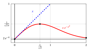
\[ \frac{1}{\sqrt{2}} {\rm ~~is~the~(unique)~global~ maximum~point~~~and~~~} 0 {\rm ~~is~the~(unique)~global~minimum~point} \]

\[ \frac{1}{\sqrt{2\: e}} {\rm ~~is~the~global~maximum~~~and~~~} 0 {\rm ~~is~the~global~minimum} \]

5.1 From the discrete to the continuous¶

Passing “from the discrete to the continuous” for sequences (i.e., from the natural numbers to the reals) is a way to make the tools of differential calculus available

Example 8: proving monotonicity of sequences by passing to the continuous

Consider the sequence

\[ a_n = \frac{\log n}{n}, {\rm ~~~~we~have~}~~a_n \ge 0, \forall n \in \N_{>0} {\rm ~~and~~} a_n \rr 0 {\rm ~~for~~} n \rr \ip \]

To prove that the sequence is eventually monotone non-increasing, one way is to use the definition and prove that:

\[ a_n \ge a_{n+1} ,~~~ \forall n \in \N_{>0} {\rm ~~~~~i.e.~~~~~~} \frac{\log n}{n} \ge \frac{\log (n+1)}{n+1},~~~ \forall n \in \N_{>0} \]

Since both the numerator and the denominator grow as \(n\) grows, it is not easy to prove this inequality algebraically.

We pass from the discrete to the continuous and define the function

\[ f(x) = \frac{\log x}{x},~~~ \forall x > 1 \]

We have

\[ f'(x) = \frac{1-\log x}{x^2} \le 0,~~~ \forall x \ge e \]

and it follows that \(f\) is non-increasing \(\forall x \ge e\). Consequently the sequence \(a_n\) is non-increasing for \(n \ge 3\) (the first natural number \(> e\)).

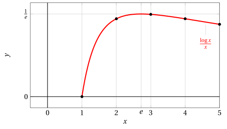
Be careful not to use the passage from the discrete to the continuous indiscriminately. For example, it cannot be done for the sequences \(\frac{n!}{2^n}\) or \(\frac{n^2+(-1)^n \; n}{n^3+1}\), since they are defined only for natural numbers.