Computing limits of functions
Part 3 · Limits of functions and continuity · Chapter 2 · lecture notes by Fabio Furini ·
1. Computing limits of functions
We state the theorems on limits of functions that follow immediately from the corresponding theorems on limits of sequences and from the sequential definition of limit
1.1 Algebra of limits theorem
Theorem 1: Algebra of limits, case of finite limits
Hypotheses as \(x \rr c\) :
\[
\textbf{1.} ~~ f(x) \rr \ell_1 \in \R, \qquad \textbf{2.} ~~ g(x) \rr \ell_2 \in \R.
\]
Thesis as \(x \rr c\) :
\[
\textbf{1.} ~~ f(x)\pm g(x) \rr \ell_1 \pm \ell_2, \qquad \textbf{2.} ~~ f(x) \: g(x) \rr \ell_1 \: \ell_2,
\]
\[
\textbf{3.} ~~ \frac{f(x)}{g(x)} \rr \frac{\ell_1}{\ell_2} ~~~~~~( \ell_2 \neq 0, g(x) \neq 0, {\rm ~~eventually~as~~} x \rr c).
\]
Proof
Let \(\{x_n\}\) be any sequence such that
\[
x_n \neq c, \forall n, {\rm ~~and~~} x_n \rr c {\rm ~~as~~} n \rr +\infty.
\]
By hypothesis we have
\[
f(x_n) \rr \ell_1 {\rm ~~and~~} g(x_n) \rr \ell_2 ~~~ (\ell_1,\ell_2 \in \R).
\]
From the theorem on the algebra of limits for sequences we therefore conclude that
\[
f(x_n) \pm g(x_n) \rr \ell_1 \pm \ell_2,
\]
and hence
\[
f(x) \pm g(x) \rr \ell_1 \pm \ell_2.
\]
Claims 2 and 3 of the theorem are proved in a perfectly analogous way. □
1.2 Sign-preservation theorems
In the following statements \(\ell\) and \(c\) will be points of \(\R^*\) unless otherwise stated.
Theorem 2: Sign preservation, \(1^{st}\) form
Hypotheses:
\[
\textbf{1.} ~~f(x) \rr \ell {\rm ~~as~~} x \rr c, \qquad \textbf{2.} ~~ \ell \lessgtr 0.
\]
Thesis:
\[
f(x) \lessgtr 0 {\rm ~~eventually~as~} x \rr c.
\]
Proof
Let \(\{x_n\}\) be any sequence such that
\[
x_n \neq c, \forall n, {\rm ~~and~~} x_n \rr c {\rm ~~as~~} n \rr +\infty
\]
By the hypothesis we have
\[
f(x_n) \rr \ell > 0
\]
hence, by the sign-preservation theorem for sequences, applied to the sequence \(\big\{f(x_n)\big\}\) , we conclude that
\[
f(x_n) > 0, ~~~~{\rm eventually}.
\]
Since this holds for every sequence such that \(x_n \rr c\) , we conclude that
\[
f(x) > 0, {\rm ~~eventually,~as~~} x \rr c
\]
□
Theorem 3: Sign preservation for functions, \(2^{nd}\) form
Hypotheses:
\[
\textbf{1.} ~~ f(x) \rr \ell \in \R {\rm ~~as~~} x \rr c,
\]
\[
\textbf{2.} ~~ f(x)\ge 0 {\rm ~~eventually~as~~} x \rr c.
\]
Thesis:
\[
\ell \ge 0.
\]
Proof
It follows from the corresponding theorem for sequences. □
For functions we also have the following sign-preservation theorem.
Theorem 4: Sign preservation for continuous functions
Hypotheses:
\[
\textbf{1.} ~~ f {\rm ~~is~continuous~at~~} c \in \R, \qquad \textbf{2.} ~~ f(c)>0.
\]
Thesis:
\[
f(x)>0 {\rm ~~eventually~as~~} x \rr c.
\]
Proof
If \(f\) is continuous at \(c\) , then
\[
f(c) = \lim_{x \rr c} f(x)
\]
hence the hypothesis \(f(c)>0\) means that
\[
f(c) = \lim_{x \rr c} f(x) > 0
\]
and this, by the sign-preservation theorem (\(1^{st}\) form), implies that
\[
f(x) > 0 {\rm ~~eventually~as~~} x \rr c.
\]
□
1.3 Comparison theorem
Theorem 5: Comparison theorem
Hypotheses:
\[
\textbf{1.} ~~ f(x) \rr \ell {\rm ~~and~~} g(x) \rr \ell {\rm ~~as~~} x \rr c,
\]
\[
\textbf{2.} ~~ f(x) \le h(x) \le g(x) {\rm ~~eventually~as~~} x \rr c.
\]
Thesis:
\[
h(x) \rr \ell {\rm ~~as~~} x \rr c.
\]
Proof
Let \(\{x_n\}\) be any sequence such that
\[
x_n \neq c, \forall n, {\rm ~~and~~} x_n \rr c {\rm ~~as~~} n \rr +\infty
\]
We want to prove that
\[
h(x_n) \rr \ell {\rm ~~as~~} n \rr +\infty
\]
By hypothesis we know that:
\[
f(x_n) \le h(x_n) \le g(x_n), {\rm ~~eventually,}
\]
\[
f(x_n) \rr \ell {\rm~~and~~} g(x_n) \rr \ell, {\rm ~~as~~} x_n \rr c
\]
Hence, by the comparison theorem for sequences applied to:
\[
\big\{f(x_n)\big\},~~ \big\{h(x_n)\big\}~~ {\rm and~~} \big\{g(x_n)\big\}
\]
we conclude that
\[
h(x_n) \rr \ell {\rm ~~as~~} n \rr +\infty
\]
□
Corollary 1: Of the comparison theorem (part I)
Hypotheses:
\[
\textbf{1.} ~~ g(x) \rr 0 {\rm ~~as~~} x \rr c,
\]
\[
\textbf{2.} ~~ |h(x)| \le g(x) {\rm ~~eventually~as~~} x \rr c.
\]
Thesis:
\[
h(x) \rr 0 {\rm ~~as~~} x \rr c.
\]
Proof
It follows from the corresponding corollary for sequences. □
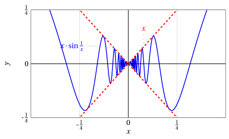
Example 1: Corollary of the comparison theorem
Let us prove that:
\[
\lim_{x \rr 0} x \: \sin \frac{1}{x} = 0
\]
We have
\[
x \rr 0 {\rm ~~as~~} x \rr 0 {\rm ~~and~~} \lim_{x \rr 0} \sin \frac{1}{x} {\rm ~~does~not~exist~}
\]
hence we cannot apply Theorem Theorem 1 on the algebra of limits for functions.
We have
\[
\left|\sin \frac{1}{x}\right| \le 1 {\rm~~hence~~} \left|x \: \sin \frac{1}{x}\right| \le |x| {\rm ~~and~~} |x| \rr 0 {\rm ~~as~~} x \rr 0.
\]
Hence, by Corollary Corollary 1 of the comparison theorem for functions, we have:
\[
x \: \sin \frac{1}{x} \rr 0 {\rm ~~as~~} x \rr 0.
\]
Corollary 2: Of the comparison theorem (part II)
Hypotheses:
\[
\textbf{1.} ~~ f(x) \rr 0 {\rm ~~as~~} x \rr c,
\]
\[
\textbf{2.} ~~ g(x) {\rm ~~is~bounded,~eventually,~as~~} x \rr c.
\]
Thesis:
\[
f(x) \: g(x) \rr 0 {\rm ~~as~~} x \rr c.
\]
Proof
It follows from the corresponding corollary for sequences. □
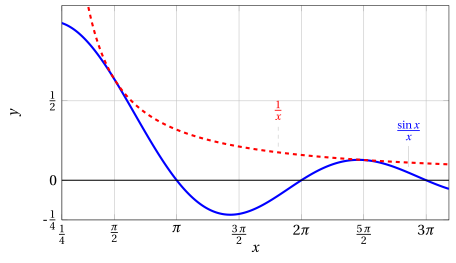
Example 2: Corollary of the comparison theorem
Let us prove that:
\[
\lim_{x \rr \ip} \frac{x + \sin x}{2\: x + \cos x}= \frac{1}{2}
\]
Factoring, we obtain
\[
\frac{x + \sin x}{2\: x + \cos x} = \frac{x \left( 1+ \frac{\sin x}{x} \right)}{2\:x \left( 1+ \frac{\cos x}{2\:x} \right)} = \frac{1}{2} \left(\frac{ 1+ \frac{\sin x}{x} }{ 1+ \frac{\cos x}{2\:x} } \right)
\]
By Corollary Corollary 2 of the comparison theorem for functions, we have:
\[
\frac{\sin x}{x} \rr 0 {\rm ~~and~~} \frac{\cos x}{2\: x} \rr 0 {\rm ~~as~~} x \rr \ip.
\]
Then, by Theorem Theorem 1 on the algebra of limits, we therefore have:
\[
\frac{x + \sin x}{2\: x + \cos x} \rr \frac{1}{2} {\rm ~~as~~} x \rr \ip.
\]
1.4 Theorems of partial arithmetization of the infinity symbol
Theorem 6: Partial arithmetization of the infinity symbol (addition)
Hypotheses as \(x \rr c\) :
\[
\textbf{1.} ~~ f(x) \rr \ell \in \R, \qquad \textbf{2.} ~~ g(x) \rr \ip, \qquad \textbf{3.} ~~ h(x) \rr \ip.
\]
Thesis as \(x \rr c\) :
\[
\textbf{1.} ~~ f(x) + g(x) \rr \ell \ip = \ip, \qquad \textbf{2.} ~~ f(x) - g(x) \rr \ell \im = \im,
\]
\[
\textbf{3.} ~~ g(x) + h(x) \rr \ip \ip = \ip, \qquad \textbf{4.} ~~ -g(x) - h(x) \rr \im \im = \im.
\]
Proof
It follows from the corresponding theorem for sequences. □
Theorem 7: Partial arithmetization of the infinity symbol (product)
Hypotheses as \(x \rr c\) :
\[
\textbf{1.} ~~ f(x) \rr \ell \in \R, \qquad \textbf{2.} ~~ g(x) \rr 0, \qquad \textbf{3.} ~~ h(x) \rr \infty.
\]
Thesis as \(x \rr c\) :
\[
\textbf{1.} ~~ f(x) \:\: h(x) \rr \ell \cdot \infty = \infty \quad (\ell \neq 0),
\qquad
\textbf{2.} ~~ \frac{f(x)}{g(x)} \rr \frac{\ell}{0} = \infty \quad (\ell \neq 0),
\]
\[
\textbf{3.} ~~ \frac{f(x)}{h(x)} \rr \frac{\ell}{\infty} = 0.
\]
Proof
It follows from the corresponding theorem for sequences. □
As for sequences, the sign of \(\infty\) must be determined with the rule of signs .
Example 3: Partial arithmetization of the infinity symbol
\[
\lim_{x \rr \im} \left(\frac{1}{x} - 2\right) \: x^3 = \ip
\]
Since \(\left(\frac{1}{x} - 2\right) \rr -2 {\rm ~~and~~} x^3 \rr \im \quad {\rm as~~} x \rr \im\) .
2. Change of variable theorem for limits
Theorem 8: Change of variable in the limit
Let \(f\) and \(g\) be two functions for which the composition \(f \circ g\) is defined, at least eventually as \(x \rr x_0 \in \R^*.\) If:
\[
1.~~~ \lim_{x \rr x_0} g(x) = t_0 \in \R^*,~~~2.~~~ \lim_{t \rr t_0} f(t) = \ell \in \R^*
\]
\[
3.~~~ g(x) \neq t_0, {\rm ~~~eventually,~as~~~} x \rr x_0
\]
Then:
\[
\lim_{x \rr x_0} f\big(g(x)\big) = \lim_{t \rr t_0} f(t).
\]
Hypothesis \(3.\) is not necessary when \(f\) is continuous at \(t_0\) , or when \(t_0= \pm \infty\) .
Proof
Let \(\{x_n\}\) be any sequence such that
\[
x_n \neq x_0, \forall n, {\rm ~~and~~} x_n \rr x_0 {\rm ~~as~~} n \rr +\infty.
\]
We have
\[
g(x_n) \rr t_0 {\rm ~~as~~} n \rr +\infty ~~({\rm by~hypothesis}~1)
\]
and
\[
g(x_n) \neq t_0, {\rm ~~eventually~~} ~({\rm by~hypothesis}~3).
\]
Therefore
\[
f\big(g(x_n)\big) \rr \ell ~~({\rm by~hypothesis}~2).
\]
If \(t_0= \pm \infty\) the condition \(g(x) \neq \pm \infty\) is obviously satisfied, while if \(f\) is continuous at \(t_0\) , \(\ell = f(t_0)\) , so if \(g(x_n)= t_0\) for some \(n\) we would have
\[
f\big(g(x_n)\big)= f(t_0)= \ell
\]
and hence the convergence
\[
f\big(g(x_n)\big) \rr \ell {\rm ~~as~~} n \rr +\infty
\]
would be guaranteed anyway. □
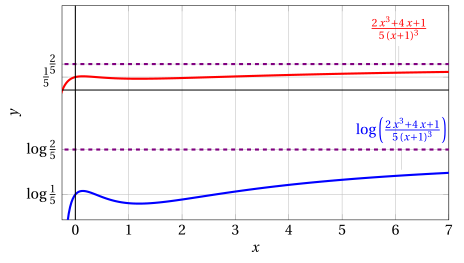
Example 4: Computing a limit with the change of variable theorem
Let us compute the limit
\[
\lim_{x \rr \ip} \log \left ( \frac{2\:x^3+4\:x+1}{5\:(x+1)^3} \right)
\]
The functions \(f\) and \(g\) are:
\[
g(x) = \left ( \frac{2\:x^3+4\:x+1}{5\:(x+1)^3} \right) {\rm ~~~~and~~~~} f(t) = \log t.
\]
We have \(t=g(x)\) and
\[
(f \circ g)(x) = f\big(g(x)\big) = \log \left ( \frac{2\:x^3+4\:x+1}{5\:(x+1)^3} \right) ~~~~{\rm and ~~~~} x_0 = \ip.
\]
We compute
\[
\lim_{x \rr \ip} g(x) = \frac{2}{5} ~~~~{\rm and ~consequently~~~} t_0 = \frac{2}{5}.
\]
Now we compute
\[
\lim_{t \rr 2/5} \log t = \log{\frac{2}{5}} \quad({\rm as~we~will~see,~the~logarithm~is ~continuous~in~} \R_+)
\]
Hence
\[
\lim_{x \rr \ip} f\big(g(x)\big) = \log{\frac{2}{5}}
\]
Moreover:
\[
\lim_{x \rr 0} f\big(g(x)\big)=\log{\frac{1}{5}}
\]
using the theorem we have:
\[
\lim_{x \rr 0} g(x) = \frac{1}{5} {\rm ~~~and~~~} \lim_{t \rr 1/5} \log t = \log{\frac{1}{5}}
\]
since
\[
\lim_{x \rr 0} 2\:x^3+4\:x+1 = 1 {\rm ~~~and~~~} \lim_{x \rr 0} 5\:(x+1)^3= 5
\]
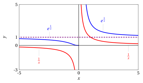
Example 5: Computing a limit with the change of variable theorem
Let us compute the limits
\[
\lim_{x \rr 0^+} e^{\frac{1}{x}} {\rm ~~~~and~~~~} \lim_{x \rr 0^-} e^{\frac{1}{x}}.
\]
The functions \(f\) and \(g\) are:
\[
g(x) = \frac{1}{x} {\rm ~~~~and~~~~} f(t) = e^t.
\]
We have \(t=g(x)\) and
\[
(f \circ g) (x) = f\big(g(x)\big) = e^{\frac{1}{x}}~~~~{\rm moreover ~~~~} x_0 = 0^+ {\rm ~~~~and~~~~} x_0 = 0^-.
\]
\(\frac{1}{x} \rr \ip\) as \(x \rr 0^+\) and hence \(t_0=\ip\) . Now we compute:
\[
\lim_{t \rr \ip} e^t = \ip {\rm ~~~~hence~~~~}
\lim_{x \rr 0^+} e^{\frac{1}{x}} = \ip.
\]
\(\frac{1}{x} \rr \im\) as \(x \rr 0^-\) and hence \(t_0=\im\) . Now we compute:
\[
\lim_{t \rr \im} e^t = 0 {\rm ~~~~hence~~~~} \lim_{x \rr 0^-} e^{\frac{1}{x}} = 0.
\]