Number sets and intervals¶

Part 2 · Numbers · Chapter 2 · Lecture notes, volume 2 (PDF) · Exercises, volume 2 (PDF) · Slides (PDF)

1. The five main number sets¶

1.1 The natural numbers¶

\(\N\) is the set of natural numbers, that is, the numbers used for counting:

\[ \N = \{0,~ 1,~ 2,~ 3,~ 4,~ \dots\} \]

We recall the convention adopted in these notes: zero is a natural number, that is \(0 \in \N\). Other textbooks exclude zero from \(\N\): it is only a convention, but it must be stated once and for all.
We denote by \(\N_{>0}\) the set of positive natural numbers:

\[ \N_{>0} = \N \setminus \{0\} = \{1,~ 2,~ 3,~ 4,~ \dots\} \]

In the chapter Sets we have already introduced, for the natural numbers:

the definitions of even number (\(n = 2\,m\)) and odd number (\(n = 2\,m+1\)), with \(m \in \N\), and the fact that every natural number is either even or odd, but never both;
the well-ordering axiom, stating that every non-empty subset of \(\N\) has a minimum.

1.2 The integers¶

\(\Z\) is the set of integers (also called signed numbers), that is:

\[ 0,~ 1,~ - 1,~ 2,~ -2,~ \dots \]

1.3 The rational numbers¶

\(\Q\) is the set of rational numbers, that is, of the fractions:

\[ \frac{n}{m},~~ {\rm~where~~} n, m \in \Z , {\rm ~~and~~} m \neq 0. \]

Rational numbers can also be written in decimal form. For example:

\[\begin{align*} \frac{3}{4} = 0.75, {\rm ~~~while~~~} \frac{1}{3} = 0.333 \dots {\rm }= 0.\overline{3}. \end{align*}\]

A rational number, written in decimal form, has a finite or infinite periodic decimal expansion: after the decimal point there is a finite number of digits, or an infinite number of digits which, from a certain point on, repeat periodically.

The same rational number can have two different decimal expansions. The classical example is the equality

\[ 0.\overline{9}=1 \]

for which we gave four different proofs in the chapter Sets, and which we therefore do not repeat here.

1.4 The real numbers¶

\(\R\) is the set of real numbers, that is, those which are identified with finite or infinite decimal expansions, periodic or non-periodic: after the decimal point there may be any string of digits, possibly infinite and non-periodic.

That numbers of this last kind exist (that is, real but not rational), can be understood by reflecting on examples such as:

\[ 0.10110111011110 \dots \]

After the decimal point, the previous number has: one digit equal to \(1\), then \(0\), then two digits equal to \(1\), then \(0\), then three digits equal to \(1\) … and so on. It is clear that this rule defines a decimal number precisely. On the other hand, the string of digits after the decimal point is neither finite nor periodic: therefore this number is irrational.

1.5 The complex numbers¶

\(\C\) is the set of complex numbers, that is, numbers of the form \(a + i\:b\), where \(a\), \(b\) are real numbers, and \(i\) is the imaginary unit, that is, a number whose square is \(-1\).

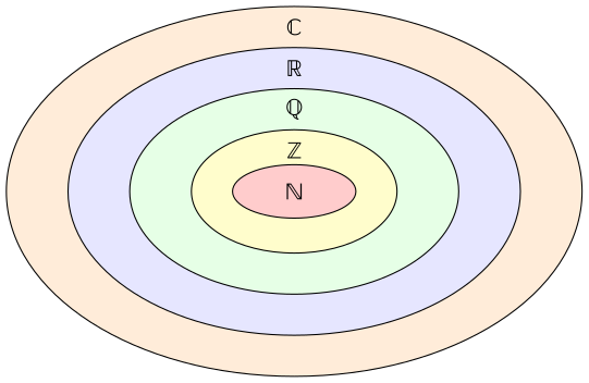
Among the number sets introduced, the following inclusions hold:

\[ \N ~\subsetneqq~ \Z ~\subsetneqq~ \Q ~\subsetneqq~ \R ~\subsetneqq~ \C. \]

As indicated by the symbols, all the inclusions are strict:

there exist integers that are not natural numbers (the negative numbers),
there exist rational numbers that are not integers (the proper fractions),
there exist real numbers that are not rational (the irrational numbers),
there exist complex numbers that are not real (the imaginary numbers).

As for \(\N_{>0}\), we denote by

\[ \Z_{>0}, \qquad \Q_{>0}, \qquad \R_{>0} \]

the sets of positive integer, rational and real numbers, and by

\[ \Z_{\ge 0}, \qquad \Q_{\ge 0}, \qquad \R_{\ge 0} \]

the sets of non-negative integer, rational and real numbers (that is, positive or zero). For example:

\[ \R_{>0} = \{x \in \R : x > 0\} \qquad {\rm ~~and~~} \qquad \Z_{\ge 0} = \{x \in \Z : x \ge 0\} = \N \]

2. Intervals¶

Definition 1: of bounded interval

Given two real numbers \(a\), \(b\), a bounded interval with endpoints \(a\) and \(b\) is one of the following sets:

\[\begin{align*} [a,b] = \big\{ x \in \mathbb{R}: a \le x \le b \big\}, & \qquad [a,b) = \big\{ x \in \mathbb{R}: a \le x < b \big\} \\[2ex] (a,b] = \big\{ x \in \mathbb{R}: a < x \le b \big\}, &\qquad (a,b) = \big\{ x \in \mathbb{R}: a < x < b \big\} \end{align*}\]

As can be seen, the square (round) bracket at one of the two endpoints indicates that this endpoint is included in (excluded from) the interval.
The intervals \([a, b]\) are called closed; the intervals \((a, b)\) are called open.

Definition 2: of unbounded interval

Given a real number \(a\), an unbounded interval (or half-line) with endpoint \(a\) is one of the following sets:

\[\begin{align*} [a,+\infty) = \big\{ x \in \mathbb{R}: x \ge a \big\}, & \qquad (a,+\infty) = \big\{ x \in \mathbb{R}: x > a \big\} \\[2ex] (-\infty,a] = \big\{ x \in \mathbb{R}: x \le a \big\}, &\qquad (-\infty,a) = \big\{ x \in \mathbb{R}: x < a \big\} \end{align*}\]

The symbols \(-\infty\) and \(+\infty\) are not real numbers: they are not endpoints that can belong to the set, and therefore next to them one always writes a round bracket.
The whole line is an unbounded interval as well:

\[ \mathbb{R} = (-\infty, +\infty) \]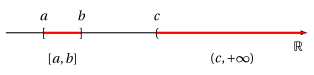

Example 1: of intervals

The graphical representation of the closed bounded interval \([-3,-2]\) and of the open unbounded interval \((2,+\infty)\) is the following:

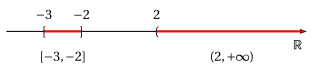
The first one contains both of its endpoints, the second one does not contain its endpoint \(2\) and is not bounded above.

It can be proved that the intervals, bounded or unbounded, are exactly the subsets \(I\) of \(\mathbb{R}\) that satisfy the following property (called connectedness):

\[ \forall x_1, x_2, x_3 \in \R {\rm ~~such~that~~} x_1 < x_2 < x_3, {\rm ~~if~~} x_1,x_3 \in I, {\rm ~~then~~} x_2 \in I \]

In what follows we will sometimes consider the Cartesian product of two (or more) intervals, which can be given the geometric meaning of a rectangle (in two dimensions) or of a parallelepiped (in three dimensions).

Example 2: Cartesian product of intervals

Let \(A = [0, 1]\), \(B = [1, 2]\); the figure

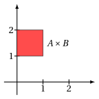
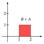
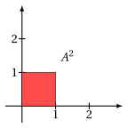
illustrates the sets \(A \times B\) , \(B \times A\) , \(A \times A\), also denoted by \(A^2\). In general, \(A \times B\) is different from \(B \times A\).