Integer part and fractional part functions
Part 3 · Functions · Chapter 7 · Lecture notes, volume 3 (PDF) · Exercises, volume 3 (PDF) · Slides (PDF)
1. Integer part and fractional part functions
- Two functions that are typically encountered when writing algorithms are the integer part (floor) function and the fractional part (or decimal part) function.
Definition 1: of the integer part function
The integer part (floor) function is:
Definition 2: of the upper integer part function
The upper integer part (ceiling) function is:
Definition 3: of the fractional part function
The fractional part function is:
-
The integer part function \(f(x)= \lfloor x \rfloor\) and the upper integer part function \(f(x)= \lceil x \rceil\) are non-decreasing in \(\mathbb{R}\), but they are not increasing.
-
They are non-decreasing: let \(x_1 < x_2\). Then \(\lfloor x_1 \rfloor \le x_1 < x_2\) and, since \(\lfloor x_1 \rfloor\) is an integer less than or equal to \(x_2\), while \(\lfloor x_2 \rfloor\) is the largest integer less than or equal to \(x_2\) (see the chapter “Roots, powers, logarithms and modular arithmetic” of Part 2), we have \(\lfloor x_1 \rfloor \le \lfloor x_2 \rfloor\). In the same way \(\lceil x_2 \rceil \ge x_2 > x_1\) and, since \(\lceil x_1 \rceil\) is the smallest integer greater than or equal to \(x_1\), we have \(\lceil x_1 \rceil \le \lceil x_2 \rceil\).
-
They are not increasing: both are constant on every interval between two consecutive integers, for instance
\[ \left\lfloor \frac{1}{3} \right\rfloor = \left\lfloor \frac{2}{3} \right\rfloor = 0 \qquad {\rm ~~and~~} \qquad \left\lceil \frac{1}{3} \right\rceil = \left\lceil \frac{2}{3} \right\rceil = 1, \]hence there exist \(x_1 < x_2\) with \(f(x_1) = f(x_2)\).
-
-
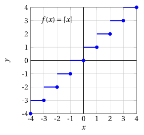
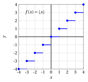
Graphs of the functions \(f(x)=\lceil x \rceil\) and \(f(x)= \lfloor x \rfloor\) on the interval \([-4,4]\).
-
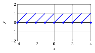
Note that the fractional part is a periodic function with period 1:
2. Piecewise-defined functions
- Starting from the elementary functions, new ones can be built by using different analytic definitions on different intervals.
Definition 4: of piecewise-defined function
A function \(f\) whose value \(f (x)\) is computed through different “instructions” depending on the interval in which \(x\) lies is called a piecewise-defined function.
Example 1: Piecewise-defined functions
Consider for example
its graph is:
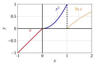
- From the logical / algorithmic point of view, one can say that a function of this kind has the peculiarity of being built using not only mathematical functions but also the logical function “if … then”.
3. The absolute-value function
-
In the chapter “Factorials, binomial coefficients and triangle inequality” of Part 2 the absolute value of a real number \(a\) was defined by
\[ |a| = \begin{cases} a & {\rm if~~} a \ge 0\\ -a & {\rm if~~} a < 0 \end{cases} \]Associating with every \(x \in \mathbb{R}\) the number \(|x|\) we obtain a function of a real variable, which is the most important example of a piecewise defined function.
Definition 5: of absolute-value function
The absolute-value function is:
-
Sign. The absolute-value function is nonnegative in \(\mathbb{R}\) and positive in \(\mathbb{R} \setminus \{0\}\):
\[ |x| \ge 0,~~ \forall x \in \mathbb{R} \qquad {\rm ~~and~~} \qquad |x| = 0 ~~\Longleftrightarrow~~ x=0. \]Indeed, if \(x \ge 0\) then \(|x|=x \ge 0\), and if \(x<0\) then \(|x|=-x>0\); in both cases \(|x|=0\) forces \(x=0\).
-
Monotonicity. The absolute-value function is decreasing in \((-\infty,0]\) and increasing in \([0,+\infty)\), but it is not monotonic in \(\mathbb{R}\).
-
If \(x_1 < x_2 \le 0\), then \(|x_1| = -x_1 > -x_2 = |x_2|\).
-
If \(0 \le x_1 < x_2\), then \(|x_1| = x_1 < x_2 = |x_2|\).
-
It is not monotonic in \(\mathbb{R}\) because \(f(-1)=1 > f(0)=0\) (hence it is not non-decreasing in \(\mathbb{R}\)) and \(f(0)=0 < f(1)=1\) (hence it is not non-increasing in \(\mathbb{R}\)).
-
-
Boundedness and image. The function is bounded below in \(\mathbb{R}\) (the number \(0\) is a lower bound for its values), but it is not bounded above: for every \(M \in \R\) with \(M>0\) we have \(f(M+1)=M+1>M\). Its image is
\[ f(\mathbb{R}) = [0,+\infty), \]because \(|x| \ge 0\) for every \(x\) and, conversely, every \(y \ge 0\) is the image of \(y\) itself: \(|y|=y\).
-
Symmetry. The absolute-value function is even, since \(|-x|=|x|\) for every \(x \in \mathbb{R}\): its graph is symmetric with respect to the \(y\)-axis.
-
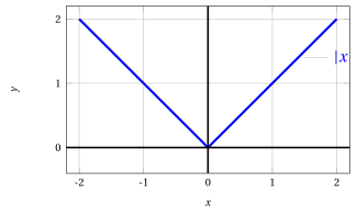
The graph consists of the two half-lines \(y=-x\) for \(x \le 0\) and \(y=x\) for \(x \ge 0\):