30.6 Scheduling on parallel machines: longest jobs first
Part 4 · Heuristic algorithms · Chapter 30 · Chapter 30: Constructive heuristics · Lecture notes, volume 4 (PDF) · Slides (1/2) · Slides (2/2) · Exercises: Constructive heuristics · App: Bin packing heuristics · App: List scheduling and LPT · App: Vertex coloring: greedy and DSATUR · App: TSP: nearest neighbour and 2-opt
- For \(P\,||\,C_{\max}\) the elements are the assignments of jobs to machines, and every assignment is feasible. A natural greedy rule assigns each job to the machine that is currently least loaded, so that the loads grow as evenly as possible. As for the BPP, the rule chooses the machine, and the order of the jobs is a second, independent, choice.
30.6.1 List scheduling
The List Scheduling Algorithm (denoted by \(LIST\)) is a constructive heuristic for \(P\,||\,C_{\max}\). It examines the jobs in the order of a given list \(\rho\) and assigns each job to a machine with the smallest current load (in case of ties, the machine with the smallest index).
Algorithm: List Scheduling
-
\(LIST\) is the scheduling counterpart of an online rule: it does not need to know the future jobs, and it is used, for example, when jobs arrive one at a time. With a linear scan of the machines it runs in \(O(nm)\) time, and in \(O(n\log m)\) time with a heap of the loads.
-
On the reference instance, \(t=(5,5,4,4,3,3,3)\), the jobs are listed by non-increasing processing time, which is a favourable order. To see the effect of the order, the example examines the same jobs in the reverse list.
Example 30.5: \(LIST\) on the reference instance, shortest jobs first
Consider the list \(\rho=(7,6,5,4,3,2,1)\), i.e., the jobs by non-decreasing processing time. The loads before each assignment and the chosen machine are:
| job \(j\) | \(t_j\) | loads \((L_1,L_2,L_3)\) before | machine |
|---|---|---|---|
| \(7\) | \(3\) | \((0,0,0)\) | \(1\) |
| \(6\) | \(3\) | \((3,0,0)\) | \(2\) |
| \(5\) | \(3\) | \((3,3,0)\) | \(3\) |
| \(4\) | \(4\) | \((3,3,3)\) | \(1\) |
| \(3\) | \(4\) | \((7,3,3)\) | \(2\) |
| \(2\) | \(5\) | \((7,7,3)\) | \(3\) |
| \(1\) | \(5\) | \((7,7,8)\) | \(1\) |
The final loads are \((12,7,8)\), with \(J_1=\{7,4,1\}\), \(J_2=\{6,3\}\), \(J_3=\{5,2\}\), and \(LIST(I)=12\):
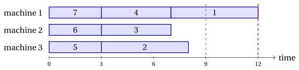
The last job of the list is one of the longest: when it arrives, the least loaded machine already has load \(7\), and the makespan jumps to \(12\), three units above the lower bound \(9\) (dashed grey line).
Proposition 30.3
For every \(P\,||\,C_{\max}\) instance \(I\) and every list \(\rho\),
Proof
Proof omitted. The result is due to
R.L. Graham, Bounds for certain multiprocessing anomalies, Bell System Technical Journal 45 (1966) 1563–1581. □
\(LIST\) is a \(\left(2-\frac{1}{m}\right)\)-approximation algorithm for \(P\,||\,C_{\max}\), whatever the order of the list.
- On the example, \(LIST(I)=12\le \frac{5}{3}\cdot 9=15\).
30.6.2 Longest processing time first
The Longest Processing Time first Algorithm (denoted by \(LPT\)) is a constructive heuristic for \(P\,||\,C_{\max}\). It sorts the jobs by non-increasing processing time and applies \(LIST\) to this list: each job, from the longest to the shortest, is assigned to a least loaded machine.
Algorithm: Longest Processing Time first
-
Why the longest jobs first. The makespan is decided by the job that finishes last. If the jobs are short at the end of the list, the last assignments can only add a little to the least loaded machine, and they act as “sand” that levels the loads. The parallel with FFD is exact: the large elements first, the small ones to fill the gaps.
-
\(LPT\) runs in \(O(n\log n + n\log m)\) time.
Example 30.6: \(LPT\) on the reference instance
The jobs are already sorted, \(\rho=(1,2,3,4,5,6,7)\). Jobs \(1\), \(2\), \(3\) go to the three empty machines, with loads \((5,5,4)\); job \(4\) goes to machine \(3\), the least loaded: \((5,5,8)\); job \(5\) goes to machine \(1\): \((8,5,8)\); job \(6\) to machine \(2\): \((8,8,8)\); job \(7\) finds three machines with load \(8\) and goes to machine \(1\): \((11,8,8)\). Hence \(J_1=\{1,5,7\}\), \(J_2=\{2,6\}\), \(J_3=\{3,4\}\), \(mach=(1,2,3,3,1,2,1)\), and \(LPT(I)=11\):
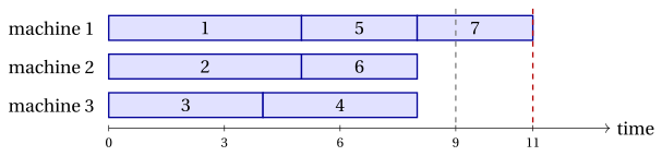
The elementary lower bound of the chapter «Heuristic algorithms: definitions» gives \(z(I)\ge\max\left\{\max_j t_j,\left\lceil\frac{\sum_j t_j}{m}\right\rceil\right\}=\max\{5,9\}=9\), and \(z(I)=9\). Sorting improves the makespan from \(12\) to \(11\), but \(LPT\) is not optimal: after six jobs the loads are perfectly balanced, \((8,8,8)\), and the seventh job unbalances them by \(3\).
Proposition 30.4
For every \(P\,||\,C_{\max}\) instance \(I\),
Proof
Proof omitted. The result is due to
R.L. Graham, Bounds on multiprocessing timing anomalies, SIAM Journal on Applied Mathematics 17 (1969) 416–429. □
\(LPT\) is a \(\left(\frac{4}{3}-\frac{1}{3m}\right)\)-approximation algorithm for \(P\,||\,C_{\max}\): sorting the list lowers the guarantee of \(LIST\) from \(2-\frac{1}{m}\) to \(\frac{4}{3}-\frac{1}{3m}\).
-
For \(m=3\) the bound is \(\frac{4}{3}-\frac{1}{9}=\frac{11}{9}\), and on the reference instance
\[ \frac{LPT(I)}{z(I)}=\frac{11}{9}. \]The reference instance attains Graham's bound exactly: it belongs to the family of instances, given by Graham, with \(2m+1\) jobs of processing times \(2m-1,2m-1,2m-2,2m-2,\dots,m+1,m+1,m,m,m\), on which \(LPT\) gives \(4m-1\) and the optimum is \(3m\). For \(m=3\) these are the times \((5,5,4,4,3,3,3)\). The bound of Proposition 30.4 therefore cannot be improved.
Next: 30.7 The travelling salesman problem: append or insert?