DP for the capacitated lot sizing problem
Part 3 · Dynamic programming · Chapter 26 · Lecture notes, volume 3 (PDF) · Slides · Exercises: Capacitated lot sizing (CLS)
Prerequisites
-
From this module, the chapter «DP for the uncapacitated lot sizing problem»: the total demands \(D_{j,t}\), the encoding of a production plan and its network, the zero-inventory ordering property, and the instance of its Example 25.1.
-
From this module, the chapters «Lot sizing problems» and «Formulations of lot sizing problems»: the capacitated problem, its reference instance, and its ILP model with the variables \(x_t\), \(s_t\), \(y_t\).
-
From this module, the chapter «Principles of dynamic programming»: recurrence, base cases, lookup table and reconstruction of a solution.
-
From the module Algorithms: pseudocode (Chapter 2), and the size of the input (Chapter 11).
Where we were
-
As a problem and as a model: the capacitated lot sizing problem and its ILP formulations (Chapter 8 «Lot sizing problems» and Chapter 15 «Formulations of lot sizing problems»).
-
As a table, without capacities: the DP algorithm of Wagner and Whitin of Chapter 25 «DP for the uncapacitated lot sizing problem», over the production runs, in \(\Theta(m^2)\) steps.
-
Now, with capacities: a DP algorithm on the pairs (period, inventory), which is pseudo-polynomial.
Objectives
At the end of this chapter you will be able to:
-
explain why the zero-inventory ordering property fails with capacities, on an example;
-
write the recurrence \(v(t,k)\) on the pairs (period, final inventory), with its base cases;
-
run the DP algorithm by hand, fill the matrices \({v}\) and \({r}\), and reconstruct an optimal plan;
-
count the steps of the DP algorithm, and say why it is pseudo-polynomial;
-
state the weaker property that holds when the capacity is the same in all periods.
The problem of this chapter is the capacitated lot sizing problem (CLS): its definition and its assumptions are on its page.
26.1 Notation, model and feasible solutions
-
As in Chapter 25 «DP for the uncapacitated lot sizing problem», for any \(j,t \in T\) we denote by
\[ D_{j,t}=\sum_{k=j}^{t} d_k \]the total demand of periods \(j,j+1,\dots,t\), with \(D_{j,t}=0\) if \(j>t\).
-
The ILP model is the \(\mathrm{ILP}_{\mathrm{CLSP}}\) model of Chapter 15 «Formulations of lot sizing problems», with the big-M value \(\min\{cap_t, D_{t,m}\}\) of period \(t\): it is the \(\mathrm{ILP}_{\mathrm{ULS}}\) model with the additional constraints \(x_t\le cap_t\), for all \(t\in T\).
-
A feasible solution is encoded by the same vector \((x_1,x_2,\dots,x_m)\) as in the ULS, with the inventories \(s_t=\sum_{j=1}^{t} x_j-D_{1,t}\), and with the additional requirement \(x_t \le cap_t\) for all \(t\in T\).
-
The zero-inventory ordering property does not hold for the CLS: a period may have to produce while units are still in stock, because the capacity does not allow to produce everything in the period where it would be cheapest.
-
The property, and the DP algorithm over the production runs that rests on it, are those of Chapter 25 «DP for the uncapacitated lot sizing problem».
Example 26.1: Capacitated lot sizing
We consider the uncapacitated instance of Example 25.1 of Chapter 25 «DP for the uncapacitated lot sizing problem», measured in units of \(10\) products (hence the holding cost is \(10\) per unit), with a constant capacity of \(4\) units per period:
We refer to this CLS instance as Example 26.1: it is the reference instance of Chapter 8 «Lot sizing problems». The optimal solution of the uncapacitated instance, in units of \(10\), is the vector \((3,\allowbreak 0,\allowbreak 8,\allowbreak 0,\allowbreak 0)\), of cost \(170\): it is not feasible for Example 26.1, since period \(3\) produces more than \(4\) units.
26.2 A DP algorithm for the CLS
26.2.1 Step 1 and Step 2
-
Step 1: computation of the optimal value
-
For any period \(t\in\{1,\dots,m\}\), the production cost function of period \(t\) is
\[ f_t(x)= \left\{ \begin{array}{ll} 0 & \textrm{if $x=0$,}\\[1ex] sc_t+vc_t\,x & \textrm{if $x\in\{1,2,\dots,cap_t\}$.} \end{array} \right. \]The inventory at the end of period \(t\) never exceeds the demand \(D_{t+1,m}\) of the following periods, since the inventory must be empty at the end of period \(m\).
For any \(t \in \{1,2,\dots,m\}\) and \(k \in \{0,1,\dots,D_{t+1,m}\}\), let \(v(t,k)\) be the optimal value of the CLS subinstance given by:
-
a set \(\{1,2,\dots,t\}\) of \(t\) time periods,
-
for each period \(j \in \{1,2,\dots,t\}\), a demand \(d_j\),
-
for each period \(j \in \{1,2,\dots,t\}\), a setup cost \(sc_j\), a variable production cost \(vc_j\), and a holding cost \(hc_j\),
-
for each period \(j \in \{1,2,\dots,t\}\), a capacity \(cap_j\),
-
an inventory equal to \(k\) at the end of period \(t\).
The recursive formula to compute \(v(t,k)\) reads as follows:
\[\begin{equation*} \label{eq:cls} v(t,k)= \left\{ \begin{array}{ll} \begin{array}[t]{@{}l@{}}\displaystyle \min \bigg\{ v(t-1,k+d_t-x) + f_t(x) : x \in X_t(k)\bigg\}\\ {}+ hc_t\,k\end{array} & \textrm{if $1\le t \le m$,}\\[2ex] 0 & \textrm{if $t=0$ and $k=0$,}\\[2ex] +\infty & \textrm{if $t=0$ and $k>0$,} \end{array} \right. \tag{26.1} \end{equation*}\]where \(X_t(k)=\{0,1,\dots,\min\{cap_t,\,k+d_t\}\}\) is the set of the possible productions of period \(t\).
-
The pair \((t,k)\) is the state: the last period of the subinstance and the inventory at its end. For \(t=m\) and \(k=0\) we obtain the CLS instance itself, so its optimal value is \(v(m,0)\).
-
The recursive decomposition process of formula \(\eqref{eq:cls}\) generates at most \(cap_t+1\) independent subproblems, each corresponding to a possible choice of the production \(x\) of the last period \(t\).
-
If \(x\) units are produced in period \(t\) and \(k\) units remain at its end, the inventory at the end of period \(t-1\) is \(k+d_t-x\): the residual subproblem is the CLS subinstance with periods \(\{1,\dots,t-1\}\) and final inventory \(k+d_t-x\).
-
The production \(x\) is at most \(cap_t\), and at most \(k+d_t\) because the inventory at the end of period \(t-1\) cannot be negative. Moreover \(k+d_t-x\le D_{t+1,m}+d_t=D_{t,m}\), so the residual subproblem is a state.
-
The base case is \(v(0,0)=0\): no period, no inventory, no cost.
-
For \(k>0\) we set \(v(0,k)=+\infty\): the initial inventory is empty, so no feasible solution has a positive inventory before period \(1\). The value \(+\infty\) rules out this case, and it propagates to every state that cannot be reached within the capacities, with the convention \(+\infty+a=+\infty\).
-
The optimal value \(v(t,k)\) is obtained by trying all possible productions \(x\) of period \(t\) and selecting the one that minimizes the sum \(v(t-1,k+d_t-x)+f_t(x)\) of the optimal value of the residual subproblem and the production cost of period \(t\); the holding cost \(hc_t\,k\) of the final inventory does not depend on \(x\).
-
Hence, an optimal solution of the subinstance of state \((t,k)\) is built by combining the chosen production of period \(t\) with an optimal solution of the residual subproblem of state \((t-1,k+d_t-x)\).
\(\rightsquigarrow\) Optimal Substructure verified!
-
Different sequences of production decisions can lead to the same state. For instance, in Example 26.1, starting from the state \((5,0)\), the decisions \(x_5=0\) and \(x_4=4\) lead to the state \((3,1)\), and the decisions \(x_5=1\) and \(x_4=3\) lead to the same state \((3,1)\).
-
Therefore the same value \(v(t,k)\) may need to be computed several times during the recursive evaluation of formula \(\eqref{eq:cls}\).
\(\rightsquigarrow\) Overlapping Subproblems verified!
-
A first method to compute the optimal value \(v(m,0)\) of the CLS instance is the top-down approach. The method starts from the call with \((t,k)=(m,0)\) and evaluates formula \(\eqref{eq:cls}\) recursively: each call for a state \((t,k)\) triggers further calls for the states \((t-1,k+d_t-x)\), for all \(x \in \{0,\dots,\min\{cap_t,k+d_t\}\}\), until one of the base cases \(v(0,k)\) is reached.
-
The value \(v(t,k)\) can be computed once the values \(v(t-1,k')\) are known for all \(k'\in\{0,\dots,D_{t,m}\}\).
-
We can avoid solving the same subproblems repeatedly by storing the value of each subproblem as soon as it is computed, in a lookup table: the matrix \({v}[0..m][0..D_{1,m}]\), whose cell \({v}[t][k]\) contains \(v(t,k)\) for \(k\le D_{t+1,m}\) (the other cells are not used).
-
A second method to compute the optimal value \(v(m,0)\) of the CLS instance is the bottom-up approach. The method starts from the base cases \(v(0,0)=0\) and \(v(0,k)=+\infty\) for all \(k\in\{1,\dots,D_{1,m}\}\).
-
It evaluates formula \(\eqref{eq:cls}\) for increasing values of \(t\in\{1,\dots,m\}\) and, for each fixed \(t\), for \(k \in \{0,1,\dots,D_{t+1,m}\}\): each value \(v(t,k)\) uses already-computed values of row \(t-1\), until \(v(m,0)\) is obtained.
This is the pseudo-code of the DP algorithm using the bottom-up approach:
Algorithm: DP_CLS
Input: A CLS instance given by the number \(m\) of periods and the arrays \(d[1..m]\), \(sc[1..m]\), \(vc[1..m]\), \(hc[1..m]\), \(cap[1..m]\)Output: The optimal value1Function DP_CLS(\(m,d,sc,vc,hc,cap\))2\({R} := \textnormal{new array}[0..m]\)3\({R}[m] \leftarrow 0\)4for \(t := m-1\) downto \(0\) do5\({R}[t] \leftarrow {R}[t+1] + d[t+1]\)6end7\({v} := \textnormal{new array}[0..m][0..{R}[0]]\)8\({v}[0][0] \leftarrow 0\)9for \(k := 1\) to \({R}[0]\) do10\({v}[0][k] \leftarrow +\infty\)11end12for \(t := 1\) to \(m\) do13for \(k := 0\) to \({R}[t]\) do14\(\mathit{b} := +\infty\)15for \(x := 0\) to \(\min\{cap[t],\,k+d[t]\}\) do16if \({v}[t-1][k+d[t]-x] + f_t(x) + hc[t]\cdot k < \mathit{b}\) then17\(\mathit{b} \leftarrow {v}[t-1][k+d[t]-x] + f_t(x) + hc[t]\cdot k\)18end19end20\({v}[t][k] \leftarrow \mathit{b}\)21end22end23return \({v}[m][0]\)-
The vector \({R}[0..m]\) contains the remaining demands \({R}[t]=D_{t+1,m}\), computed backwards from \({R}[m]=0\): the states of period \(t\) are the pairs \((t,k)\) with \(k\le {R}[t]\).
-
The matrix \({v}\) is the lookup table. The initialization sets \({v}[0][0]=0\) and \({v}[0][k]=+\infty\) for all \(k\in\{1,\dots,{R}[0]\}\), since the initial inventory is empty.
-
The outer loop, over \(t \in \{1,2,\dots,m\}\), considers the periods in increasing order, and the second loop, over \(k\in\{0,\dots,{R}[t]\}\), considers all final inventories of period \(t\).
-
The inner loop, over the production \(x\) of period \(t\), keeps in \(\mathit{b}\) the smallest value \({v}[t-1][k+d[t]-x]+f_t(x)+hc[t]\cdot k\); the value \(f_t(x)\) is \(0\) for \(x=0\) and \(sc[t]+vc[t]\cdot x\) otherwise. If all candidates are \(+\infty\), the comparison is never true and \({v}[t][k]=+\infty\): the state \((t,k)\) cannot be reached within the capacities.
-
Finally, the optimal value \({v}[m][0]\) of the CLS instance is returned.
Example 26.2: Execution of the DP algorithm
We consider the CLS instance of Example 26.1:
\[ \begin{array}{l|rrrrr} \hline {t} & {1} & {2} & {3} & {4} & {5} \\ \hline {d_t} & {2} & {1} & {3} & {4} & {1} \\ {sc_t} & {50} & {50} & {50} & {50} & {50} \\ {vc_t} & {0} & {0} & {0} & {0} & {0} \\ {hc_t} & {10} & {10} & {10} & {10} & {10} \\ {cap_t} & {4} & {4} & {4} & {4} & {4} \\ \hline \end{array} \]The remaining demands are \(({R}[0],\dots,{R}[5])=(11,\allowbreak 9,\allowbreak 8,\allowbreak 5,\allowbreak 1,\allowbreak 0)\).
For each step of the DP algorithm, the table shows the values of \(t\) and \(k\), the cell \({v}[t][k]\), and the operation performed. The candidates of the minimum are listed for \(x=0,1,\dots,\min\{cap_t,k+d_t\}\).
\(t\) \(k\) \({v}[t][k]\) Action \(0\) \(0\) \(0\) \({v}[0][0]\leftarrow 0\) \(0\) \(1\) \(+\infty\) \({v}[0][1]\leftarrow +\infty\) \(0\) \(2\) \(+\infty\) \({v}[0][2]\leftarrow +\infty\) \(0\) \(3\) \(+\infty\) \({v}[0][3]\leftarrow +\infty\) \(0\) \(4\) \(+\infty\) \({v}[0][4]\leftarrow +\infty\) \(0\) \(5\) \(+\infty\) \({v}[0][5]\leftarrow +\infty\) \(0\) \(6\) \(+\infty\) \({v}[0][6]\leftarrow +\infty\) \(0\) \(7\) \(+\infty\) \({v}[0][7]\leftarrow +\infty\) \(0\) \(8\) \(+\infty\) \({v}[0][8]\leftarrow +\infty\) \(0\) \(9\) \(+\infty\) \({v}[0][9]\leftarrow +\infty\) \(0\) \(10\) \(+\infty\) \({v}[0][10]\leftarrow +\infty\) \(0\) \(11\) \(+\infty\) \({v}[0][11]\leftarrow +\infty\) \(1\) \(0\) \(50\) \(\min\{{v}[0][2]{+}f_{1}(0),\allowbreak {v}[0][1]{+}f_{1}(1),\allowbreak {v}[0][0]{+}f_{1}(2)\}{+}hc_{1}\cdot 0\) \(=\min\{+\infty,\allowbreak +\infty,\allowbreak 0{+}50\}{+}10\cdot 0=50\) \(1\) \(1\) \(60\) \(\min\{{v}[0][3]{+}f_{1}(0),\allowbreak {v}[0][2]{+}f_{1}(1),\allowbreak {v}[0][1]{+}f_{1}(2),\allowbreak {v}[0][0]{+}f_{1}(3)\}{+}hc_{1}\cdot 1\) \(=\min\{+\infty,\allowbreak +\infty,\allowbreak +\infty,\allowbreak 0{+}50\}{+}10\cdot 1=60\) \(1\) \(2\) \(70\) \(\min\{{v}[0][4]{+}f_{1}(0),\allowbreak {v}[0][3]{+}f_{1}(1),\allowbreak {v}[0][2]{+}f_{1}(2),\allowbreak {v}[0][1]{+}f_{1}(3),\allowbreak {v}[0][0]{+}f_{1}(4)\}{+}hc_{1}\cdot 2\) \(=\min\{+\infty,\allowbreak +\infty,\allowbreak +\infty,\allowbreak +\infty,\allowbreak 0{+}50\}{+}10\cdot 2=70\) \(1\) \(3\) \(+\infty\) the candidates use the cells \({v}[0][1],\dots,{v}[0][5]\), which are all \(+\infty\): \({v}[1][3]\leftarrow +\infty\) \(1\) \(4\) \(+\infty\) the candidates use the cells \({v}[0][2],\dots,{v}[0][6]\), which are all \(+\infty\): \({v}[1][4]\leftarrow +\infty\) \(1\) \(5\) \(+\infty\) the candidates use the cells \({v}[0][3],\dots,{v}[0][7]\), which are all \(+\infty\): \({v}[1][5]\leftarrow +\infty\) \(1\) \(6\) \(+\infty\) the candidates use the cells \({v}[0][4],\dots,{v}[0][8]\), which are all \(+\infty\): \({v}[1][6]\leftarrow +\infty\) \(1\) \(7\) \(+\infty\) the candidates use the cells \({v}[0][5],\dots,{v}[0][9]\), which are all \(+\infty\): \({v}[1][7]\leftarrow +\infty\) \(1\) \(8\) \(+\infty\) the candidates use the cells \({v}[0][6],\dots,{v}[0][10]\), which are all \(+\infty\): \({v}[1][8]\leftarrow +\infty\) \(1\) \(9\) \(+\infty\) the candidates use the cells \({v}[0][7],\dots,{v}[0][11]\), which are all \(+\infty\): \({v}[1][9]\leftarrow +\infty\) \(2\) \(0\) \(60\) \(\min\{{v}[1][1]{+}f_{2}(0),\allowbreak {v}[1][0]{+}f_{2}(1)\}{+}hc_{2}\cdot 0\) \(=\min\{60{+}0,\allowbreak 50{+}50\}{+}10\cdot 0=60\) \(2\) \(1\) \(80\) \(\min\{{v}[1][2]{+}f_{2}(0),\allowbreak {v}[1][1]{+}f_{2}(1),\allowbreak {v}[1][0]{+}f_{2}(2)\}{+}hc_{2}\cdot 1\) \(=\min\{70{+}0,\allowbreak 60{+}50,\allowbreak 50{+}50\}{+}10\cdot 1=80\) \(2\) \(2\) \(120\) \(\min\{{v}[1][3]{+}f_{2}(0),\allowbreak {v}[1][2]{+}f_{2}(1),\allowbreak {v}[1][1]{+}f_{2}(2),\allowbreak {v}[1][0]{+}f_{2}(3)\}{+}hc_{2}\cdot 2\) \(=\min\{+\infty,\allowbreak 70{+}50,\allowbreak 60{+}50,\allowbreak 50{+}50\}{+}10\cdot 2=120\) \(2\) \(3\) \(130\) \(\min\{{v}[1][4]{+}f_{2}(0),\allowbreak {v}[1][3]{+}f_{2}(1),\allowbreak {v}[1][2]{+}f_{2}(2),\allowbreak {v}[1][1]{+}f_{2}(3),\allowbreak {v}[1][0]{+}f_{2}(4)\}{+}hc_{2}\cdot 3\) \(=\min\{+\infty,\allowbreak +\infty,\allowbreak 70{+}50,\allowbreak 60{+}50,\allowbreak 50{+}50\}{+}10\cdot 3=130\) \(2\) \(4\) \(150\) \(\min\{{v}[1][5]{+}f_{2}(0),\allowbreak {v}[1][4]{+}f_{2}(1),\allowbreak {v}[1][3]{+}f_{2}(2),\allowbreak {v}[1][2]{+}f_{2}(3),\allowbreak {v}[1][1]{+}f_{2}(4)\}{+}hc_{2}\cdot 4\) \(=\min\{+\infty,\allowbreak +\infty,\allowbreak +\infty,\allowbreak 70{+}50,\allowbreak 60{+}50\}{+}10\cdot 4=150\) \(2\) \(5\) \(170\) \(\min\{{v}[1][6]{+}f_{2}(0),\allowbreak {v}[1][5]{+}f_{2}(1),\allowbreak {v}[1][4]{+}f_{2}(2),\allowbreak {v}[1][3]{+}f_{2}(3),\allowbreak {v}[1][2]{+}f_{2}(4)\}{+}hc_{2}\cdot 5\) \(=\min\{+\infty,\allowbreak +\infty,\allowbreak +\infty,\allowbreak +\infty,\allowbreak 70{+}50\}{+}10\cdot 5=170\) \(2\) \(6\) \(+\infty\) the candidates use the cells \({v}[1][3],\dots,{v}[1][7]\), which are all \(+\infty\): \({v}[2][6]\leftarrow +\infty\) \(2\) \(7\) \(+\infty\) the candidates use the cells \({v}[1][4],\dots,{v}[1][8]\), which are all \(+\infty\): \({v}[2][7]\leftarrow +\infty\) \(2\) \(8\) \(+\infty\) the candidates use the cells \({v}[1][5],\dots,{v}[1][9]\), which are all \(+\infty\): \({v}[2][8]\leftarrow +\infty\) \(3\) \(0\) \(110\) \(\min\{{v}[2][3]{+}f_{3}(0),\allowbreak {v}[2][2]{+}f_{3}(1),\allowbreak {v}[2][1]{+}f_{3}(2),\allowbreak {v}[2][0]{+}f_{3}(3)\}{+}hc_{3}\cdot 0\) \(=\min\{130{+}0,\allowbreak 120{+}50,\allowbreak 80{+}50,\allowbreak 60{+}50\}{+}10\cdot 0=110\) \(3\) \(1\) \(120\) \(\min\{{v}[2][4]{+}f_{3}(0),\allowbreak {v}[2][3]{+}f_{3}(1),\allowbreak {v}[2][2]{+}f_{3}(2),\allowbreak {v}[2][1]{+}f_{3}(3),\allowbreak {v}[2][0]{+}f_{3}(4)\}{+}hc_{3}\cdot 1\) \(=\min\{150{+}0,\allowbreak 130{+}50,\allowbreak 120{+}50,\allowbreak 80{+}50,\allowbreak 60{+}50\}{+}10\cdot 1=120\) \(3\) \(2\) \(150\) \(\min\{{v}[2][5]{+}f_{3}(0),\allowbreak {v}[2][4]{+}f_{3}(1),\allowbreak {v}[2][3]{+}f_{3}(2),\allowbreak {v}[2][2]{+}f_{3}(3),\allowbreak {v}[2][1]{+}f_{3}(4)\}{+}hc_{3}\cdot 2\) \(=\min\{170{+}0,\allowbreak 150{+}50,\allowbreak 130{+}50,\allowbreak 120{+}50,\allowbreak 80{+}50\}{+}10\cdot 2=150\) \(3\) \(3\) \(200\) \(\min\{{v}[2][6]{+}f_{3}(0),\allowbreak {v}[2][5]{+}f_{3}(1),\allowbreak {v}[2][4]{+}f_{3}(2),\allowbreak {v}[2][3]{+}f_{3}(3),\allowbreak {v}[2][2]{+}f_{3}(4)\}{+}hc_{3}\cdot 3\) \(=\min\{+\infty,\allowbreak 170{+}50,\allowbreak 150{+}50,\allowbreak 130{+}50,\allowbreak 120{+}50\}{+}10\cdot 3=200\) \(3\) \(4\) \(220\) \(\min\{{v}[2][7]{+}f_{3}(0),\allowbreak {v}[2][6]{+}f_{3}(1),\allowbreak {v}[2][5]{+}f_{3}(2),\allowbreak {v}[2][4]{+}f_{3}(3),\allowbreak {v}[2][3]{+}f_{3}(4)\}{+}hc_{3}\cdot 4\) \(=\min\{+\infty,\allowbreak +\infty,\allowbreak 170{+}50,\allowbreak 150{+}50,\allowbreak 130{+}50\}{+}10\cdot 4=220\) \(3\) \(5\) \(250\) \(\min\{{v}[2][8]{+}f_{3}(0),\allowbreak {v}[2][7]{+}f_{3}(1),\allowbreak {v}[2][6]{+}f_{3}(2),\allowbreak {v}[2][5]{+}f_{3}(3),\allowbreak {v}[2][4]{+}f_{3}(4)\}{+}hc_{3}\cdot 5\) \(=\min\{+\infty,\allowbreak +\infty,\allowbreak +\infty,\allowbreak 170{+}50,\allowbreak 150{+}50\}{+}10\cdot 5=250\) \(4\) \(0\) \(160\) \(\min\{{v}[3][4]{+}f_{4}(0),\allowbreak {v}[3][3]{+}f_{4}(1),\allowbreak {v}[3][2]{+}f_{4}(2),\allowbreak {v}[3][1]{+}f_{4}(3),\allowbreak {v}[3][0]{+}f_{4}(4)\}{+}hc_{4}\cdot 0\) \(=\min\{220{+}0,\allowbreak 200{+}50,\allowbreak 150{+}50,\allowbreak 120{+}50,\allowbreak 110{+}50\}{+}10\cdot 0=160\) \(4\) \(1\) \(180\) \(\min\{{v}[3][5]{+}f_{4}(0),\allowbreak {v}[3][4]{+}f_{4}(1),\allowbreak {v}[3][3]{+}f_{4}(2),\allowbreak {v}[3][2]{+}f_{4}(3),\allowbreak {v}[3][1]{+}f_{4}(4)\}{+}hc_{4}\cdot 1\) \(=\min\{250{+}0,\allowbreak 220{+}50,\allowbreak 200{+}50,\allowbreak 150{+}50,\allowbreak 120{+}50\}{+}10\cdot 1=180\) \(5\) \(0\) \(180\) \(\min\{{v}[4][1]{+}f_{5}(0),\allowbreak {v}[4][0]{+}f_{5}(1)\}{+}hc_{5}\cdot 0\) \(=\min\{180{+}0,\allowbreak 160{+}50\}{+}10\cdot 0=180\) This is the matrix \({v}\) after the execution of the DP algorithm (a dot marks a pair \((t,k)\) with \(k>D_{t+1,m}\), which is not a state):
\[ \begin{array}{l|rrrrrrrrrrrr} \hline {{v}[t][k]} & {0} & {1} & {2} & {3} & {4} & {5} & {6} & {7} & {8} & {9} & {10} & {11} \\ \hline {t=0} & {0} & {+\infty} & {+\infty} & {+\infty} & {+\infty} & {+\infty} & {+\infty} & {+\infty} & {+\infty} & {+\infty} & {+\infty} & {+\infty} \\ {t=1} & {50} & {60} & {70} & {+\infty} & {+\infty} & {+\infty} & {+\infty} & {+\infty} & {+\infty} & {+\infty} & {\cdot} & {\cdot} \\ {t=2} & {60} & {80} & {120} & {130} & {150} & {170} & {+\infty} & {+\infty} & {+\infty} & {\cdot} & {\cdot} & {\cdot} \\ {t=3} & {110} & {120} & {150} & {200} & {220} & {250} & {\cdot} & {\cdot} & {\cdot} & {\cdot} & {\cdot} & {\cdot} \\ {t=4} & {160} & {180} & {\cdot} & {\cdot} & {\cdot} & {\cdot} & {\cdot} & {\cdot} & {\cdot} & {\cdot} & {\cdot} & {\cdot} \\ {t=5} & {180} & {\cdot} & {\cdot} & {\cdot} & {\cdot} & {\cdot} & {\cdot} & {\cdot} & {\cdot} & {\cdot} & {\cdot} & {\cdot} \\ \hline \end{array} \]The optimal value of the CLS instance is \({v}[5][0]=180\).
-
-
After the execution of the DP algorithm, the matrix \({v}\) contains the optimal value \({v}[t][k]\) for every state \((t,k)\).
-
-
Step 2: computation of an optimal solution
-
To compute an optimal solution, it is necessary to store some additional information.
-
For each state \((t,k)\), in addition to the optimal value \({v}[t][k]\), we store \({r}[t][k]\), the production of period \(t\) in an optimal solution of the subinstance of state \((t,k)\); for the states with value \(+\infty\) we store \(0\).
-
Starting from \((t,k)=(m,0)\), the value \({r}[t][k]\) gives the production of period \(t\); the inventory at the end of period \(t-1\) is then \(k+d_t-{r}[t][k]\), and the same rule can be applied again to period \(t-1\), and so on, until \(t=0\).
This is the pseudo-code of the DP algorithm using the bottom-up approach with the storing of the information necessary to compute an optimal solution:
Algorithm: DP_CLS_InfoSol
Input: A CLS instance given by the number \(m\) of periods and the arrays \(d[1..m]\), \(sc[1..m]\), \(vc[1..m]\), \(hc[1..m]\), \(cap[1..m]\)Output: The optimal value and the information matrix \({r}[0..m][0..D_{1,m}]\)1Function DP_CLS_InfoSol(\(m,d,sc,vc,hc,cap\))2\({R} := \textnormal{new array}[0..m]\)3\({R}[m] \leftarrow 0\)4for \(t := m-1\) downto \(0\) do5\({R}[t] \leftarrow {R}[t+1] + d[t+1]\)6end7\({v} := \textnormal{new array}[0..m][0..{R}[0]]\)8\({r} := \textnormal{new array}[0..m][0..{R}[0]]\)9\({v}[0][0] \leftarrow 0\)10\({r}[0][0] \leftarrow 0\)11for \(k := 1\) to \({R}[0]\) do12\({v}[0][k] \leftarrow +\infty\)13\({r}[0][k] \leftarrow 0\)14end15for \(t := 1\) to \(m\) do16for \(k := 0\) to \({R}[t]\) do17\(\mathit{b} := +\infty\)18\(\mathit{a} := 0\)19for \(x := 0\) to \(\min\{cap[t],\,k+d[t]\}\) do20if \({v}[t-1][k+d[t]-x] + f_t(x) + hc[t]\cdot k < \mathit{b}\) then21\(\mathit{b} \leftarrow {v}[t-1][k+d[t]-x] + f_t(x) + hc[t]\cdot k\)22\(\mathit{a} \leftarrow x\)23end24end25\({v}[t][k] \leftarrow \mathit{b}\)26\({r}[t][k] \leftarrow \mathit{a}\)27end28end29return \({v}[m][0], {r}\)- The DP algorithm uses the additional temporary variable \(\mathit{a}\) to keep track of the decision made when \(\mathit{b}\) is updated: if the production \(x\) is selected, \(\mathit{a}\leftarrow x\) stores this decision, and at the end of the inner loop \({r}[t][k]\leftarrow\mathit{a}\) stores it, together with the optimal value \({v}[t][k]\leftarrow\mathit{b}\). Because of the strict comparison, in case of ties the smallest production is stored.
Example 26.3: Computation of the additional information
We consider the CLS instance of Example 26.1:
\[ \begin{array}{l|rrrrr} \hline {t} & {1} & {2} & {3} & {4} & {5} \\ \hline {d_t} & {2} & {1} & {3} & {4} & {1} \\ {sc_t} & {50} & {50} & {50} & {50} & {50} \\ {vc_t} & {0} & {0} & {0} & {0} & {0} \\ {hc_t} & {10} & {10} & {10} & {10} & {10} \\ {cap_t} & {4} & {4} & {4} & {4} & {4} \\ \hline \end{array} \]For each step of the DP algorithm, the table shows the values of \(t\) and \(k\), the cell \({r}[t][k]\), and the production \(x\) for which the minimum of the corresponding row of Example 26.2 is attained first.
\(t\) \(k\) \({r}[t][k]\) Action \(0\) \(0\) 0 \({r}[0][0]\leftarrow 0\) \(0\) \(1\) 0 \({r}[0][1]\leftarrow 0\) \(0\) \(2\) 0 \({r}[0][2]\leftarrow 0\) \(0\) \(3\) 0 \({r}[0][3]\leftarrow 0\) \(0\) \(4\) 0 \({r}[0][4]\leftarrow 0\) \(0\) \(5\) 0 \({r}[0][5]\leftarrow 0\) \(0\) \(6\) 0 \({r}[0][6]\leftarrow 0\) \(0\) \(7\) 0 \({r}[0][7]\leftarrow 0\) \(0\) \(8\) 0 \({r}[0][8]\leftarrow 0\) \(0\) \(9\) 0 \({r}[0][9]\leftarrow 0\) \(0\) \(10\) 0 \({r}[0][10]\leftarrow 0\) \(0\) \(11\) 0 \({r}[0][11]\leftarrow 0\) \(1\) \(0\) \(2\) first minimum at \(x=2\), i.e., \({v}[0][0]{+}f_{1}(2){+}hc_{1}\cdot 0=0{+}50{+}0=50\): \({r}[1][0]\leftarrow 2\) \(1\) \(1\) \(3\) first minimum at \(x=3\), i.e., \({v}[0][0]{+}f_{1}(3){+}hc_{1}\cdot 1=0{+}50{+}10=60\): \({r}[1][1]\leftarrow 3\) \(1\) \(2\) \(4\) first minimum at \(x=4\), i.e., \({v}[0][0]{+}f_{1}(4){+}hc_{1}\cdot 2=0{+}50{+}20=70\): \({r}[1][2]\leftarrow 4\) \(1\) \(3\) \(0\) all candidates equal \(+\infty\): \({r}[1][3]\leftarrow 0\) \(1\) \(4\) \(0\) all candidates equal \(+\infty\): \({r}[1][4]\leftarrow 0\) \(1\) \(5\) \(0\) all candidates equal \(+\infty\): \({r}[1][5]\leftarrow 0\) \(1\) \(6\) \(0\) all candidates equal \(+\infty\): \({r}[1][6]\leftarrow 0\) \(1\) \(7\) \(0\) all candidates equal \(+\infty\): \({r}[1][7]\leftarrow 0\) \(1\) \(8\) \(0\) all candidates equal \(+\infty\): \({r}[1][8]\leftarrow 0\) \(1\) \(9\) \(0\) all candidates equal \(+\infty\): \({r}[1][9]\leftarrow 0\) \(2\) \(0\) \(0\) first minimum at \(x=0\), i.e., \({v}[1][1]{+}f_{2}(0){+}hc_{2}\cdot 0=60{+}0{+}0=60\): \({r}[2][0]\leftarrow 0\) \(2\) \(1\) \(0\) first minimum at \(x=0\), i.e., \({v}[1][2]{+}f_{2}(0){+}hc_{2}\cdot 1=70{+}0{+}10=80\): \({r}[2][1]\leftarrow 0\) \(2\) \(2\) \(3\) first minimum at \(x=3\), i.e., \({v}[1][0]{+}f_{2}(3){+}hc_{2}\cdot 2=50{+}50{+}20=120\): \({r}[2][2]\leftarrow 3\) \(2\) \(3\) \(4\) first minimum at \(x=4\), i.e., \({v}[1][0]{+}f_{2}(4){+}hc_{2}\cdot 3=50{+}50{+}30=130\): \({r}[2][3]\leftarrow 4\) \(2\) \(4\) \(4\) first minimum at \(x=4\), i.e., \({v}[1][1]{+}f_{2}(4){+}hc_{2}\cdot 4=60{+}50{+}40=150\): \({r}[2][4]\leftarrow 4\) \(2\) \(5\) \(4\) first minimum at \(x=4\), i.e., \({v}[1][2]{+}f_{2}(4){+}hc_{2}\cdot 5=70{+}50{+}50=170\): \({r}[2][5]\leftarrow 4\) \(2\) \(6\) \(0\) all candidates equal \(+\infty\): \({r}[2][6]\leftarrow 0\) \(2\) \(7\) \(0\) all candidates equal \(+\infty\): \({r}[2][7]\leftarrow 0\) \(2\) \(8\) \(0\) all candidates equal \(+\infty\): \({r}[2][8]\leftarrow 0\) \(3\) \(0\) \(3\) first minimum at \(x=3\), i.e., \({v}[2][0]{+}f_{3}(3){+}hc_{3}\cdot 0=60{+}50{+}0=110\): \({r}[3][0]\leftarrow 3\) \(3\) \(1\) \(4\) first minimum at \(x=4\), i.e., \({v}[2][0]{+}f_{3}(4){+}hc_{3}\cdot 1=60{+}50{+}10=120\): \({r}[3][1]\leftarrow 4\) \(3\) \(2\) \(4\) first minimum at \(x=4\), i.e., \({v}[2][1]{+}f_{3}(4){+}hc_{3}\cdot 2=80{+}50{+}20=150\): \({r}[3][2]\leftarrow 4\) \(3\) \(3\) \(4\) first minimum at \(x=4\), i.e., \({v}[2][2]{+}f_{3}(4){+}hc_{3}\cdot 3=120{+}50{+}30=200\): \({r}[3][3]\leftarrow 4\) \(3\) \(4\) \(4\) first minimum at \(x=4\), i.e., \({v}[2][3]{+}f_{3}(4){+}hc_{3}\cdot 4=130{+}50{+}40=220\): \({r}[3][4]\leftarrow 4\) \(3\) \(5\) \(4\) first minimum at \(x=4\), i.e., \({v}[2][4]{+}f_{3}(4){+}hc_{3}\cdot 5=150{+}50{+}50=250\): \({r}[3][5]\leftarrow 4\) \(4\) \(0\) \(4\) first minimum at \(x=4\), i.e., \({v}[3][0]{+}f_{4}(4){+}hc_{4}\cdot 0=110{+}50{+}0=160\): \({r}[4][0]\leftarrow 4\) \(4\) \(1\) \(4\) first minimum at \(x=4\), i.e., \({v}[3][1]{+}f_{4}(4){+}hc_{4}\cdot 1=120{+}50{+}10=180\): \({r}[4][1]\leftarrow 4\) \(5\) \(0\) \(0\) first minimum at \(x=0\), i.e., \({v}[4][1]{+}f_{5}(0){+}hc_{5}\cdot 0=180{+}0{+}0=180\): \({r}[5][0]\leftarrow 0\) This is the matrix \({r}\) after the execution of the DP algorithm:
\[ \begin{array}{l|rrrrrrrrrrrr} \hline {{r}[t][k]} & {0} & {1} & {2} & {3} & {4} & {5} & {6} & {7} & {8} & {9} & {10} & {11} \\ \hline {t=0} & {0} & {0} & {0} & {0} & {0} & {0} & {0} & {0} & {0} & {0} & {0} & {0} \\ {t=1} & {2} & {3} & {4} & {0} & {0} & {0} & {0} & {0} & {0} & {0} & {\cdot} & {\cdot} \\ {t=2} & {0} & {0} & {3} & {4} & {4} & {4} & {0} & {0} & {0} & {\cdot} & {\cdot} & {\cdot} \\ {t=3} & {3} & {4} & {4} & {4} & {4} & {4} & {\cdot} & {\cdot} & {\cdot} & {\cdot} & {\cdot} & {\cdot} \\ {t=4} & {4} & {4} & {\cdot} & {\cdot} & {\cdot} & {\cdot} & {\cdot} & {\cdot} & {\cdot} & {\cdot} & {\cdot} & {\cdot} \\ {t=5} & {0} & {\cdot} & {\cdot} & {\cdot} & {\cdot} & {\cdot} & {\cdot} & {\cdot} & {\cdot} & {\cdot} & {\cdot} & {\cdot} \\ \hline \end{array} \] -
Once the matrix \({r}\) has been computed, an optimal solution of the CLS instance can be computed by applying the following rule for \(t=m,m-1,\dots,1\), starting from \(k=0\):
\[ x_t \leftarrow {r}[t][k], \qquad k \leftarrow k+d_t-x_t. \]This yields the vector \((x_1,x_2,\dots,x_m)\), where each entry \(x_t\) is the number of units produced in period \(t\) in an optimal solution.
-
The following pseudo-code implements the computation of an optimal solution, given the matrix \({r}\).
Algorithm: DP_CLS_SolComputation
Input: The number \(m\) of periods and the demands \(d[1..m]\) of the CLS instance, and the matrix \({r}[0..m][0..D_{1,m}]\)Output: An optimal solution of the CLS instance1Function DP_CLS_SolComputation(\(m,d,{r}\))2\(x := \textnormal{new array}[1..m]\)3\(k := 0\)4for \(t := m\) downto \(1\) do5\(x[t] \leftarrow {r}[t][k]\)6\(k \leftarrow k + d[t] - x[t]\)7end8return \(x\)Example 26.4: Computing an optimal solution
After the execution of the DP algorithm on the instance of Example 26.1, we have the matrix \({r}\) of Example 26.3. We can compute an optimal solution as follows:
Iteration \(t\) \(k\) \({r}[t][k]\) \(x[1]\) \(x[2]\) \(x[3]\) \(x[4]\) \(x[5]\) \(k\leftarrow k+d[t]-x[t]\) \(-\) \(-\) \(-\) \(-\) 0 0 0 0 0 \(t=5\), \(k=0\) \(1\) \(5\) \(0\) \(0\) 0 0 0 0 0 \(k=0+1-0=1\) \(2\) \(4\) \(1\) \(4\) 0 0 0 4 0 \(k=1+4-4=1\) \(3\) \(3\) \(1\) \(4\) 0 0 4 4 0 \(k=1+3-4=0\) \(4\) \(2\) \(0\) \(0\) 0 0 4 4 0 \(k=0+1-0=1\) \(5\) \(1\) \(1\) \(3\) 3 0 4 4 0 \(k=1+2-3=0\) An optimal solution is the vector:
\[ (3,\allowbreak 0,\allowbreak 4,\allowbreak 4,\allowbreak 0) \]The setups are in periods \(1\), \(3\), \(4\), the inventories are \((s_1,\dots,s_{5})=(1,\allowbreak 0,\allowbreak 1,\allowbreak 1,\allowbreak 0)\), and the total cost is (there is no variable production cost)
\[ \underbrace{50+50+50}_{\text{setup}}+\underbrace{10\cdot 1+10\cdot 0+10\cdot 1+10\cdot 1+10\cdot 0}_{\text{holding}}=150+30=180. \]The corresponding optimal value is \({v}[5][0]=180\), the same value given by Gurobi on the \(\mathrm{ILP}_{\mathrm{CLSP}}\) model; the capacity costs \(180-170\) with respect to the uncapacitated instance. The network of the solution is:
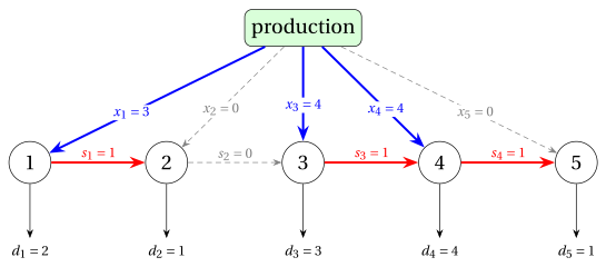
Period \(4\) produces although one unit is in stock at the end of period \(3\): the solution does not have the zero-inventory ordering property (and it is the unique optimal solution with integer quantities).
-
26.2.2 Number of steps
-
Let \(S(m,D,C)\) denote the number of steps executed by DP_CLS in the worst case, where \(m\) is the number of periods, \(D=D_{1,m}\) is the total demand, and \(C=\max_{t\in T} cap_t\) is the largest capacity. For every \(t\ge 1\) we have \({R}[t]+1\le D\) (since \(d_1\ge 1\)), and the inner loop has at most \(C+1\) iterations. In the worst case, the condition at line 16 is always true. The number of executions of the lines is:
-
Line 2, Line 3, Line 7, and Line 8 are executed \(1\) time each.
-
Line 12 is executed \(m\) times.
-
Line 13, Line 14, and Line 20 are executed \(\displaystyle\sum_{t=1}^{m}({R}[t]+1)\le mD\) times each.
-
Line 15, Line 16, and Line 17 are executed at most \(mD(C+1)\) times each.
-
Line 23 is executed \(1\) time.
Therefore,
\[ S(m,D,C)\le 5+3m+2D+3mD+3mD(C+1)=5+3m+2D+6mD+3mDC, \]and hence
\[ S(m,D,C)=O(mDC). \]The DP algorithm executes
\[ S(m,D,C)=O(m\,D\,C) \]steps in the worst case. The number of steps depends on the values \(D\) and \(C\), not only on the number \(m\) of periods: the DP algorithm is pseudo-polynomial.
-
-
DP_CLS_InfoSol only adds a constant number of operations inside the same loops, and therefore its number of steps has the same order of growth.
-
Example. Consider the capacitated instance with \(6\) periods, demands \((50,\allowbreak 30,\allowbreak 10,\allowbreak 10,\allowbreak 40,\allowbreak 10)\), setup cost \(40\), holding cost \(1\), and capacity \(80\). Measured in units of \(10\), it has \(35\) states with \(t\ge 1\).
-
The DP algorithm gives the optimal value \(160\), with the production plan \((50,\allowbreak 50,\allowbreak 0,\allowbreak 0,\allowbreak 50,\allowbreak 0)\) (in the original units): the same value given by Gurobi on the \(\mathrm{ILP}_{\mathrm{CLSP}}\) model.
26.2.3 The case of constant capacity
-
With general capacities \(cap_t\) the CLS is NP-hard, so a polynomial algorithm is not expected and the pseudo-polynomial DP algorithm is a natural exact method for small values of \(D\) and \(C\).
-
When the capacity is the same in all periods, \(cap_t=C\) for all \(t\in T\), the CLS can be solved in polynomial time, because the zero-inventory ordering property is replaced by a weaker one:
If \(cap_t=C\) for all \(t\in T\), there is an optimal solution in which, between two consecutive periods with empty inventory, at most one period produces a quantity strictly between \(0\) and \(C\); all the other periods produce \(0\) or \(C\).
-
The CLS with constant capacity has its own page in the catalogue of problems.
-
Example 26.1 has constant capacity \(C=4\). Its optimal solution \((3,\allowbreak 0,\allowbreak 4,\allowbreak 4,\allowbreak 0)\) has inventories \((1,\allowbreak 0,\allowbreak 1,\allowbreak 1,\allowbreak 0)\), empty at the end of periods \(0\), \(2\), and \(5\).
-
In periods \(1\)–\(2\) only period \(1\) produces a quantity strictly between \(0\) and \(4\), and in periods \(3\)–\(5\) every period produces \(0\) or \(4\), as stated by the property.
26.3 Typical mistakes
Warning
-
Applying the zero-inventory ordering property with capacities. With capacities a period can produce while units are in stock: in Example 26.1 the unique optimal plan violates the property.
-
Forgetting the base cases with value \(+\infty\). The initial inventory is empty, so \(v(0,k)=+\infty\) for \(k>0\); this value marks every state that cannot be reached within the capacities.
-
Allowing too large an inventory. At the end of period \(t\) the inventory is at most \(D_{t+1,m}\), since it must be empty at the end of period \(m\): the other pairs \((t,k)\) are not states.
-
Putting the holding cost inside the choice. The cost \(hc_t\,k\) of the final inventory is paid in the state \((t,k)\) whatever the production \(x\): it is added outside the minimum.
-
Calling \(O(mDC)\) polynomial. The running time contains the total demand \(D\) and the largest capacity \(C\), which are numbers of the input: the DP algorithm is pseudo-polynomial.
26.4 In summary
In summary
-
With capacities the zero-inventory ordering property fails: a period may produce while units are in stock, and the DP algorithm over the production runs does not apply.
-
The state is the pair \((t,k)\) of the period and the final inventory, with \(k\le D_{t+1,m}\); the recurrence \(v(t,k)\) chooses the production \(x\) of period \(t\), and the optimal value is \(v(m,0)\).
-
The matrix \({r}\) of the chosen productions, read backwards from the state \((m,0)\), gives an optimal plan.
-
The DP algorithm takes \(O(mDC)\) steps, which is pseudo-polynomial.
-
With a constant capacity a weaker property holds, and the problem is polynomial; with general capacities it is NP-hard.
Dashboard of the example.
| Instance | Lower bound | Upper bound | Origin |
|---|---|---|---|
| Example 26.1 (capacitated, \(C=4\)) | \(180\) | \(180\) | DP algorithm on (period, inventory) |
Exercises on this chapter: Capacitated lot sizing (CLS)