8.2 The capacitated lot sizing problem

Part 1 · Combinatorial optimization problems · Chapter 8 · Chapter 8: Lot sizing problems · Lecture notes, volume 1 (PDF) · Slides · Exercises: Lot sizing problems

Definition 8.1: Capacitated lot sizing problem

Given:

1. a set \(T = \{1,2,\dots,m\}\) of \(m\) time periods,

2. for each period \(t \in T\), a demand \(d_t \in \Z_{\ge 1}\) and a capacity \(cap_t \in \Z_{\ge 1}\), both counted in units of one product,

3. for each period \(t \in T\), three non-negative integer costs: the setup cost \(sc_t\), the variable production cost \(vc_t\) per unit produced and the holding cost \(hc_t\) per unit kept in stock at the end of the period,

the capacitated lot sizing problem (CLS) asks to decide how much to produce in every period, so that every demand is satisfied with what is produced and what is in stock, the capacities are respected, and the total cost of setups, production and holding is minimized.

• A CLS instance is specified by:

  1. one integer number:

     • the number of periods \(m \in \Z_{\ge 1}\),

  2. five vectors of integer numbers of length \(m\):

     • \(\vet{d},\ \vet{cap} \in \Z_{\ge 1}^m\), containing demands and capacities,

     • \(\vet{sc},\ \vet{vc},\ \vet{hc} \in \Z_{\ge 0}^m\), containing the costs.

• A CLS feasible solution is a production plan, that is a vector of integer quantities

  \[ \vet{x} = (x_1,x_2,\dots,x_m) \in \Z_{\ge 0}^m , \]

  where \(x_t\) is the quantity produced in period \(t\). The stock left at the end of period \(t\) is

  \[ s_t(\vet{x}) = \sum_{u=1}^{t} (x_u - d_u), \]

  because the stock of period \(t-1\) plus the production of period \(t\) must cover the demand of period \(t\), and what remains is the stock of period \(t\). The plan is feasible if

  \[ x_t \le cap_t \quad \text{and} \quad s_t(\vet{x}) \ge 0 \qquad \forall t \in T, \qquad s_m(\vet{x}) = 0. \]

• There is a setup in period \(t\) when \(x_t > 0\): we write \(y_t = 1\) in this case and \(y_t = 0\) otherwise. The cost of a plan is

  \[ c(\vet{x}) = \sum_{t \in T} \bigl( sc_t\, y_t + vc_t\, x_t + hc_t\, s_t(\vet{x}) \bigr). \]

  Given a CLS instance, the CLS can be formally stated as:

  \[\begin{equation*} \label{CLS} \tilde{\vet{x}} \in \argmin_{\vet{x}} \left\{ c(\vet{x}) \;:\; x_t \le cap_t,~ s_t(\vet{x}) \ge 0,~ \forall t \in T,~ s_m(\vet{x}) = 0,~ \vet{x} \in \Z_{\ge 0}^m \right\}. \tag{8.1} \end{equation*}\]

• We denote by \(z(I)\) the cost of an optimal plan \(\tilde{\vet{x}}\) of the instance \(I\).

Example 8.1: CLS instance

We consider \(m=5\) periods, with the following data, all integer:

period \(t\)	\(1\)	\(2\)	\(3\)	\(4\)	\(5\)
demand \(d_t\)	\(2\)	\(1\)	\(3\)	\(4\)	\(1\)
capacity \(cap_t\)	\(4\)	\(4\)	\(4\)	\(4\)	\(4\)
setup cost \(sc_t\)	\(50\)	\(50\)	\(50\)	\(50\)	\(50\)
production cost \(vc_t\)	\(0\)	\(0\)	\(0\)	\(0\)	\(0\)
holding cost \(hc_t\)	\(10\)	\(10\)	\(10\)	\(10\)	\(10\)

The total demand is \(2+1+3+4+1=11\). We call this CLS instance Example 8.1: it is the reference instance of the chapter.

The plan \(\vet{x}=(3,0,4,4,0)\) is feasible: the stocks are \(s=(1,0,1,1,0)\), all non-negative, with \(s_5=0\), and every quantity is at most \(4\). There are \(3\) setups, in the periods \(1\), \(3\) and \(4\):

\[ c(\vet{x}) = 3\cdot 50 + 10\cdot(1+0+1+1+0) = 150+30=180. \]

The plan is drawn below, period by period from left to right: the production \(x_t\) enters a period from above, through a setup (solid) or not at all (dashed); the stock \(s_t\) passes to the next period; the demand \(d_t\) leaves the period from below.

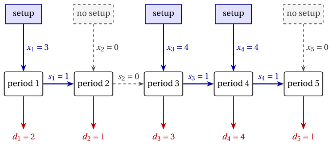
Every period has capacity \(cap_t=4\), and the three setups cost \(50\) each.

8.2.1 Assumptions

• We make the following assumptions:

  1. The stock is empty at the beginning and at the end of the horizon. Leaving stock at the end only adds cost, so no optimal plan needs it; an initial stock is a variant of the problem (Section 8.6).

  2. The capacities allow to satisfy the demands, period after period (otherwise there is no feasible plan). Formally:

     \[ \sum_{u=1}^{t} cap_u \ge \sum_{u=1}^{t} d_u, ~~~~ \forall t \in T \]

  3. The quantities are integer. With integer data, once the periods with a setup are fixed, what remains is a minimum cost flow problem, which has an integer optimal solution: restricting the quantities to integers does not change the optimal cost.

8.3 Counting the solutions

• The combinatorial part of the decision is the choice of the periods with a setup: there are \(2^m\) subsets of periods. Not all of them are feasible, because the periods with a setup must have enough capacity to produce everything.

• For a given choice of the setup periods there may be many production plans, since the quantities can be distributed in many ways: the number of feasible plans is larger than the number of feasible setup choices.

Example 8.2: counting the plans

For the instance of Example 8.1 there are \(2^5=32\) subsets of periods. Let \(k_t\) be the number of setups in the periods \(1,\dots,t\): the cumulative demands \(2,3,6,10,11\) require, with capacity \(4\), at least one setup in the periods \(1\)–\(2\), two in the periods \(1\)–\(3\) and three in the periods \(1\)–\(4\). Since \(d_1>0\) there is a setup in period \(1\), and in the periods \(2,3,4\) we need at least two setups, one of which in the periods \(2\) or \(3\):

\[ (y_2,y_3,y_4) \in \{(1,1,0),(1,0,1),(0,1,1),(1,1,1)\}. \]

The period \(5\) is free, so the feasible setup choices are \(4\cdot 2=8\) out of \(32\).

By enumeration, these setup choices carry \(94\) feasible plans. The costs of six of them are:

plan	cost	plan	cost	plan	cost
\((3,0,4,4,0)\)	\(\mathbf{180}\)	\((4,0,3,4,0)\)	\(200\)	\((2,1,4,4,0)\)	\(220\)
\((3,0,3,4,1)\)	\(210\)	\((4,0,4,3,0)\)	\(210\)	\((2,1,3,4,1)\)	\(250\)

The plan \((3,0,4,4,0)\) is the unique optimal plan, and \(z(I)=180\).

• Without the capacities the same instance has \(2^{m-1}=16\) plans that produce only when the stock is empty, and the optimal cost is \(170\): here the capacity costs \(10\).

• The optimal plan \((3,0,4,4,0)\) produces in period \(4\) with a stock of \(1\) unit, so the property of Wagner and Whitin does not hold when the capacities are binding.

• The number of setup choices grows as \(2^m\): with \(m=52\) weeks it is more than \(4\cdot 10^{15}\).

8.4 A first plan by hand

• The simplest feasible plan is lot-for-lot: in every period we produce exactly the demand of that period. There is no stock, and there are \(m\) setups; it is feasible when every demand fits in the capacity of its period.

• A plan is improved by merging: the demand of a period is produced in an earlier period, which saves a setup and costs the stock of the units anticipated.

Example 8.3: from lot-for-lot to a better plan

On the instance of Example 8.1:

1. the lot-for-lot plan \((2,1,3,4,1)\) has \(5\) setups and no stock: cost \(5\cdot 50=250\);

2. producing the demand of period \(2\) in period \(1\) saves one setup (\(-50\)) and keeps \(1\) unit for one period (\(+10\)): the plan \((3,0,3,4,1)\) costs \(210\);

3. period \(4\) cannot produce the demand of period \(5\) as well, because \(4+1>cap_4=4\); but period \(3\) can anticipate one unit of period \(4\), so that period \(4\) has room for the demand of period \(5\): the plan \((3,0,4,4,0)\) saves a setup (\(-50\)) and keeps two more units (\(+20\)).

The cost is \(210-50+20=180\).

• We have found the plan of cost \(180\) by hand, but we cannot yet tell whether a cheaper plan exists: we need a lower bound.

8.5 A combinatorial lower bound

• Let \(D=\sum_{t \in T} d_t\) be the total demand. Let \(k\) be the smallest number of periods whose capacities sum up to at least \(D\), which is found by taking the periods with the largest capacities.

Observation 8.2

For every CLS instance, every feasible plan has at least \(k\) setups, and

\[ z(I) \;\ge\; \text{the sum of the } k \text{ smallest setup costs}. \]

• The plan must produce \(D\) units in the periods with a setup, and a period without setup produces nothing: the capacities of the periods with a setup sum up to at least \(D\), hence they are at least \(k\).

• The costs of production and holding are non-negative: dropping them, and paying only \(k\) setups, the cheapest ones, gives a bound on the cost of every plan.

Example 8.4: the bound on the reference instance

For the instance of Example 8.1 we have \(D=11\) and all capacities equal to \(4\), so \(k=\lceil 11/4 \rceil = 3\). All the setup costs are \(50\), hence

\[ z(I) \ge 3 \cdot 50 = 150. \]

Together with the plans of the previous section we obtain

\[ 150 \le z(I) \le 180, \]

an absolute gap of \(30\), that is a relative gap of \(\frac{30}{150}=20\%\). The enumeration of the \(94\) plans proves that \(180\) is optimal.

---

Next: 8.6 Variants