Vertex coloring: limits of approximation

Part 5 · Approximation algorithms · Chapter 37 · Lecture notes, volume 5 (PDF) · Slides · Exercises: Vertex coloring (VCP)

Prerequisites

• From this module, the chapter «Principles of approximation algorithms»: performance ratio, \(\alpha\)-approximation algorithm, additive performance guarantee.

• From this module, the chapter «Coloring problems»: the definition of the VCP, the chromatic number \(\chi(G)\), the clique bound \(\omega(G)\le\chi(G)\) and the Petersen graph.

• From the module Algorithms (module home page): breadth-first search, polynomial time and NP-completeness.

Objectives

At the end of this chapter you will be able to:

• prove that no polynomial algorithm has a performance ratio below \(\frac43\) for the VCP, unless \(P=NP\);

• state the result of Zuckerman and explain why the VCP has no constant guarantee;

• color bipartite graphs and interval graphs optimally, and bound the colors of the greedy coloring by \(\Delta(G)+1\);

• prove that planar graphs can be colored with \(5\) colors in polynomial time, and derive an additive guarantee for them.

The problem of this chapter is the vertex coloring problem (VCP): its definition and its assumptions are on its page.

37.1 Notation

• As on the problem page, \(G=(V,E)\) is a simple graph with \(n\) vertices and \(m\) edges, \(N(v)\) is the set of the neighbours of \(v\), \(\deg(v)=|N(v)|\) its degree, and \(\Delta(G)=\max_{v\in V}\deg(v)\) the maximum degree. The optimal value of the VCP is the chromatic number, \(z(I)=\chi(G)\).

• Recall. As in the chapter «Principles of approximation algorithms», \(\mathscr{A}(I)\) is the number of colors of the coloring returned by the algorithm \(\mathscr{A}\). The VCP is a minimization problem, hence

  \[ \mathscr{A}(I) \ge \chi(G) ~~~~~~~\text{and}~~~~~~~ \frac{\mathscr{A}(I)}{\chi(G)} \ge 1 \]

  for every instance \(I\).

• Giving each vertex its own color is always feasible, so \(\chi(G)\le n\), and the ratio \(n\) is trivial. This chapter shows that a polynomial algorithm cannot do much better on all graphs, and then the classes of graphs on which it can.

37.2 The VCP is not approximable

37.2.1 No ratio below four thirds

• The proof follows the scheme of all the negative results of approximation: an algorithm with a too good guarantee would decide in polynomial time an NP-complete problem.

• The NP-complete problem is 3-colorability: given a graph \(G\), decide whether \(\chi(G)\le 3\). It remains NP-complete on planar graphs of maximum degree \(4\) (Garey, Johnson and Stockmeyer, 1976).

Theorem 37.1

Let \(\mathscr{A}\) be a polynomial algorithm for the VCP. If \(P\neq NP\), there is a graph \(G\) such that

\[ \frac{\mathscr{A}(I)}{\chi(G)} \;\ge\; \frac{4}{3} . \]

Proof

Suppose that \(\frac{\mathscr{A}(I)}{\chi(G)}<\frac43\) for every graph \(G\), and run \(\mathscr{A}\) on a graph \(G\).

1. If \(\chi(G)\le 3\), then \(\mathscr{A}(I)<\frac43\,\chi(G)\le 4\). The number of colors is an integer, hence \(\mathscr{A}(I)\le 3\).

2. If \(\chi(G)\ge 4\), then \(\mathscr{A}(I)\ge\chi(G)\ge 4\), because \(\mathscr{A}\) returns a feasible coloring.

Hence \(\chi(G)\le 3\) if and only if \(\mathscr{A}(I)\le 3\). Running \(\mathscr{A}\) and counting its colors takes polynomial time, so 3-colorability would be in \(P\), and \(P=NP\). □

• The proof uses only the integrality of \(\chi(G)\): a ratio below \(\frac43\) cannot confuse \(3\) colors with \(4\). With \(2\) colors the same argument says nothing, because deciding whether \(\chi(G)\le 2\) is easy (Section 37.3.1).

• The planar graphs of maximum degree \(4\) are a special case of the VCP: the theorem holds on them too.

37.2.2 Much stronger results

• The theorem excludes only the ratios below \(\frac43\). Much more is known, and we state it without proof.

Theorem 37.2: Zuckerman, 2007

For every \(\varepsilon>0\), if \(P\neq NP\), no polynomial algorithm \(\mathscr{A}\) for the VCP satisfies, for every graph \(G\) with \(n\) vertices,

\[ \frac{\mathscr{A}(I)}{\chi(G)} \;\le\; n^{1-\varepsilon} . \]

• The ratio \(n\) is trivial, so the chromatic number is essentially as hard to approximate as possible. The proof uses probabilistically checkable proofs and extractors.

• Earlier, Garey and Johnson (1976) had raised the bound \(\frac43\) to \(2\), and Feige and Kilian (1998) had proved the bound \(n^{1-\varepsilon}\) under a stronger assumption than \(P\neq NP\).

Corollary 37.3

If \(P\neq NP\), the VCP has no \(\alpha\)-approximation algorithm, for any constant \(\alpha\ge1\).

Proof

Let \(\mathscr{A}\) be a polynomial \(\alpha\)-approximation algorithm, and take \(\varepsilon=\frac12\). The graphs with \(n>\alpha^2\) vertices satisfy \(\frac{\mathscr{A}(I)}{\chi(G)}\le\alpha<n^{1/2}\). The graphs with \(n\le\alpha^2\) vertices are solved exactly by enumeration, in a time bounded by a constant that depends only on \(\alpha\), with ratio \(1\le n^{1/2}\). The resulting algorithm is polynomial and has ratio at most \(n^{1/2}\) on every graph, against Theorem 37.2. □

The VCP is not approximable: unless \(P=NP\), no polynomial algorithm has a constant performance guarantee, not even a guarantee of the form \(n^{1-\varepsilon}\). Positive results exist only on special classes of graphs.

37.3 Special cases

• On the four classes of this section the VCP is solved exactly, or with a guarantee, in polynomial time. The classes are recognized from the graph, or given with it (the intervals of an interval graph).

37.3.1 Bipartite graphs

Definition 37.4: bipartite graph

A graph \(G=(V,E)\) is bipartite if \(\chi(G)\le 2\), i.e., if \(V\) can be split into two stable sets.

Proposition 37.5

Deciding whether \(\chi(G)\le 2\), and finding a coloring with \(2\) colors when it exists, takes \(O(n+m)\) time.

Proof

Run a breadth-first search from a vertex of each connected component, and let \(\ell(v)\) be the level of \(v\), its distance from the root of its component. Color \(v\) with color \(1\) if \(\ell(v)\) is even and with color \(2\) otherwise.

1. If no edge joins two vertices of levels with the same parity, the coloring is feasible.

2. Otherwise, let \(\{u,v\}\) be such an edge. The paths of the search tree from the root to \(u\) and to \(v\), with the edge \(\{u,v\}\), form a closed walk of odd length \(\ell(u)+\ell(v)+1\). A closed walk of odd length contains a cycle of odd length, which needs \(3\) colors: \(\chi(G)\ge 3\).

The search and the check of the edges take \(O(n+m)\) time. □

• The proof shows the classical characterization: a graph is bipartite if and only if it has no cycle of odd length (Konig, 1936).

• On a graph with at least one edge, the search gives \(\chi(G)=2\), or the certificate \(\chi(G)\ge 3\) given by an odd cycle.

37.3.2 Graphs of bounded maximum degree

• The greedy coloring \(GC\) examines the vertices in a given order and gives each vertex the smallest color, among \(1,2,3,\dots\), not used by its neighbours already colored. It runs in \(O(n+m)\) time.

Proposition 37.6

For every graph \(G\) and every order of the vertices,

\[ GC(I) \;\le\; \Delta(G)+1 . \]

Proof

When the vertex \(v\) is colored, its neighbours already colored use at most \(\deg(v)\le\Delta(G)\) colors. One of the colors \(1,2,\dots,\Delta(G)+1\) is therefore free, and the smallest free color is at most \(\Delta(G)+1\). □

• The bound compares \(GC(I)\) with \(\Delta(G)+1\), not with \(\chi(G)\): on all graphs it is not a performance guarantee, because \(\Delta(G)\) can be \(n-1\) while \(\chi(G)=2\) (a star).

• On the graphs of maximum degree at most a fixed constant \(\Delta\), it is one. Every graph with an edge has \(\chi(G)\ge 2\), hence

  \[ \frac{GC(I)}{\chi(G)} \;\le\; \frac{\Delta+1}{2} . \]

• The bound \(\Delta(G)+1\) is attained by complete graphs and by cycles of odd length, whatever the order.

• Remark (Brooks, 1941). A connected graph that is neither complete nor a cycle of odd length satisfies \(\chi(G)\le\Delta(G)\), and such a coloring can be found in linear time.

37.3.3 Planar graphs

• A graph is planar if it can be drawn in the plane without crossing edges. Whether a graph is planar, and a drawing when it is, can be found in linear time (Hopcroft and Tarjan, 1974).

Lemma 37.7

Every planar graph with \(n\ge 3\) vertices has \(m\le 3n-6\) edges, and a vertex of degree at most \(5\).

Proof

Adding edges to a drawing without creating crossings does not decrease \(m\), so we may assume that no such edge can be added: the drawing is connected and every face is a triangle. Euler's formula for a connected planar drawing with \(f\) faces gives \(n-m+f=2\). Every face has \(3\) edges and every edge borders \(2\) faces, so \(3f=2m\), and

\[ 2 = n-m+f \;=\; n-m+\frac{2m}{3} \qquad\Longrightarrow\qquad m\le 3n-6 . \]

The degrees sum to \(2m\le 6n-12<6n\), so some vertex has degree at most \(5\). □

Theorem 37.8: Heawood, 1890

Every planar graph can be colored with \(5\) colors, and such a coloring can be found in polynomial time.

Proof

By induction on \(n\); graphs with \(n\le 5\) are trivial. Let \(v\) be a vertex of degree at most \(5\) (Lemma 37.7), and color \(G-v\), which is planar, with \(5\) colors.

1. If the neighbours of \(v\) use at most \(4\) colors, \(v\) takes the fifth one.

2. Otherwise \(v\) has \(5\) neighbours \(v_1,\dots,v_5\), in this order around \(v\) in the drawing, with colors \(1,\dots,5\). Let \(H_{13}\) be the graph induced by the vertices of colors \(1\) and \(3\).

3. If \(v_1\) and \(v_3\) are in different components of \(H_{13}\), exchange the colors \(1\) and \(3\) in the component of \(v_1\): the coloring stays feasible, and color \(1\) becomes free for \(v\).

4. Otherwise a path of colors \(1\) and \(3\) joins \(v_1\) to \(v_3\); with \(v\), it closes a cycle that separates \(v_2\) from \(v_4\) in the drawing. A path from \(v_2\) to \(v_4\) must cross that cycle, so \(v_2\) and \(v_4\) are in different components of \(H_{24}\): exchanging \(2\) and \(4\) in the component of \(v_2\) frees color \(2\) for \(v\).

Each step uses a search in \(O(n+m)=O(n)\) time, and there are \(n\) steps: \(O(n^2)\) time in total. □

• Remark (the four color theorem). Every planar graph can be colored with \(4\) colors (Appel and Haken, 1977). The proof uses a computer; Robertson, Sanders, Seymour and Thomas (1997) simplified it and gave an algorithm that finds such a coloring in \(O(n^2)\) time.

• The algorithm \(PL\) for planar graphs combines the previous results: if \(G\) has no edge, it uses \(1\) color; if \(G\) is bipartite, it uses \(2\) colors (Proposition 37.5); otherwise it uses the \(5\) colors of Theorem 37.8.

Corollary 37.9

\(PL\) is a polynomial \(2\)-additive approximation algorithm for the VCP on planar graphs:

\[ PL(I)-\chi(G) \;\le\; 2 . \]

With the four color algorithm in place of the five color one, the additive error is at most \(1\).

Proof

In the first two cases \(PL\) is exact. In the third case \(G\) has a cycle of odd length, so \(\chi(G)\ge 3\), while \(PL(I)\le 5\): the additive error is at most \(5-3=2\). With \(4\) colors it is at most \(4-3=1\). □

• The additive error \(1\) cannot be improved to \(0\): deciding whether a planar graph has \(\chi(G)\le 3\) is NP-complete. For the same reason, the ratio \(\frac43\) of the four color version is the best possible on planar graphs (Theorem 37.1).

37.3.4 Interval graphs

Definition 37.10: interval graph

A graph \(G=(V,E)\) is an interval graph if every vertex \(v\) is associated with a closed interval \([a_v,b_v]\) of the real line, and \(\{u,v\}\in E\) if and only if the two intervals intersect.

• Interval graphs describe requests over time that conflict when they overlap: lectures that need a room, reservations that need a resource. A color is a room.

Proposition 37.11

On an interval graph, the greedy coloring with the vertices in order of non-decreasing left endpoint \(a_v\) uses \(\omega(G)\) colors. It is therefore optimal: \(GC(I)=\omega(G)=\chi(G)\).

Proof

Let \(v\) be a vertex that receives color \(k\). The colors \(1,\dots,k-1\) are used by neighbours \(u\) of \(v\) colored before \(v\), so with \(a_u\le a_v\).

1. Since \([a_u,b_u]\) intersects \([a_v,b_v]\) and \(a_u\le a_v\), we have \(b_u\ge a_v\): the point \(a_v\) lies in the interval of each of these neighbours, and in the interval of \(v\).

2. The \(k\) intervals that contain \(a_v\) pairwise intersect, so their vertices form a clique and \(k\le\omega(G)\).

Hence \(GC(I)\le\omega(G)\le\chi(G)\le GC(I)\), by the clique bound. □

• Sorting the intervals takes \(O(n\log n)\) time, and the coloring \(O(n+m)\).

• The order matters: with another order the greedy coloring may use more than \(\omega(G)\) colors on an interval graph (Example 37.2).

37.4 Examples

Example 37.1: The special cases on the Petersen graph

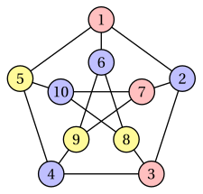
The reference instance of the VCP is the Petersen graph, with \(n=10\), \(m=15\) and \(\Delta(G)=3\).

• Is it bipartite? The search from vertex \(1\) gives the levels \(0\) to vertex \(1\), \(1\) to the vertices \(2,5,6\), and \(2\) to the other six. The edge \(\{3,4\}\) joins two vertices of level \(2\): with the paths \(1,2,3\) and \(1,5,4\) it closes the odd cycle \(1,2,3,4,5\), so \(\chi(G)\ge 3\).

• Greedy coloring. In the order \(1,2,\dots,10\), \(GC\) gives the colors \(1,2,1,2,3,2,1,3,3,2\) (red, blue, yellow in the figure): \(GC(I)=3\le\Delta(G)+1=4\).

• Together, \(3\le\chi(G)\le GC(I)=3\): the greedy coloring is optimal on this instance.

Example 37.2: The greedy coloring on an interval graph

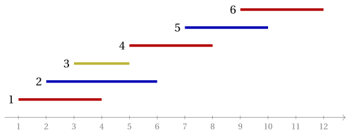
Six intervals, with the edges between intersecting intervals:

\[ [a_v,b_v]:\ [1,4],\ [2,6],\ [3,5],\ [5,8],\ [7,10],\ [9,12], \]

\[ E=\big\{\{1,2\},\{1,3\},\{2,3\},\{2,4\},\{3,4\},\{4,5\},\{5,6\}\big\}. \]

• The left endpoints are already in increasing order. \(GC\) gives the colors \(1,2,3,1,2,1\) (red, blue, yellow in the figure): \(GC(I)=3\).

• The intervals \(1,2,3\) contain the point \(3\), so \(\{1,2,3\}\) is a clique and \(\omega(G)=3\): the coloring is optimal, as Proposition 37.11 guarantees.

• With the order \(1,2,3,5,4,6\) the colors are \(1,2,3\), then \(1\) to vertex \(5\) and \(4\) to vertex \(4\), whose neighbours \(2,3,5\) use the colors \(1,2,3\): \(4\) colors, one more than \(\chi(G)\).

37.5 Sources

• M.R. Garey, D.S. Johnson, L. Stockmeyer, Some simplified NP-complete graph problems, Theoretical Computer Science 1(3):237–267, 1976.

• M.R. Garey, D.S. Johnson, The complexity of near-optimal graph coloring, Journal of the ACM 23(1):43–49, 1976.

• U. Feige, J. Kilian, Zero knowledge and the chromatic number, Journal of Computer and System Sciences 57(2):187–199, 1998.

• D. Zuckerman, Linear degree extractors and the inapproximability of max clique and chromatic number, Theory of Computing 3:103–128, 2007.

• R.L. Brooks, On colouring the nodes of a network, Proceedings of the Cambridge Philosophical Society 37(2):194–197, 1941.

• P.J. Heawood, Map-colour theorem, Quarterly Journal of Pure and Applied Mathematics 24, 1890.

• J. Hopcroft, R. Tarjan, Efficient planarity testing, Journal of the ACM 21(4):549–568, 1974.

• K. Appel, W. Haken, Every planar map is four colorable, Illinois Journal of Mathematics 21, 1977.

• N. Robertson, D. Sanders, P. Seymour, R. Thomas, The four-colour theorem, Journal of Combinatorial Theory, Series B 70(1):2–44, 1997.

37.6 Typical mistakes

Warning

• Calling the bound \(\Delta(G)+1\) a performance guarantee. It compares the greedy coloring with \(\Delta(G)+1\), not with \(\chi(G)\); it becomes a constant ratio only on graphs of bounded maximum degree.

• Reading the theorem of \(\frac43\) as an upper bound. It says that ratios below \(\frac43\) are impossible, not that a ratio of \(\frac43\) is achievable: by the result of Zuckerman, no constant ratio is.

• Using the four color theorem as an exact algorithm. It colors every planar graph with at most \(4\) colors, but deciding whether \(3\) colors suffice remains NP-complete on planar graphs.

• Sorting the intervals by right endpoint, or by length. Proposition 37.11 uses the order of the left endpoints: the colors used before \(v\) all contain the point \(a_v\).

• Forgetting the odd cycle. A breadth-first search that finds a conflict proves \(\chi(G)\ge 3\) only through the odd cycle it closes; the cycle is the certificate.

37.7 In summary

In summary

• Unless \(P=NP\), no polynomial algorithm colors every graph with fewer than \(\frac43\chi(G)\) colors: it would decide 3-colorability. By the result of Zuckerman, not even the ratio \(n^{1-\varepsilon}\) is possible: the VCP is not approximable.

• Bipartite graphs and interval graphs are colored optimally in polynomial time; on graphs of bounded degree the greedy coloring has the ratio \(\frac{\Delta+1}{2}\); on planar graphs the additive error is at most \(2\), or \(1\) with the four color theorem.

graphs	algorithm	result
all graphs	any polynomial	no constant ratio, unless \(P=NP\)
bipartite	breadth-first search	exact, \(O(n+m)\)
maximum degree \(\le\Delta\)	greedy coloring	at most \(\Delta+1\) colors
planar	\(PL\)	additive error \(\le 2\) (or \(\le 1\))
interval	greedy by left endpoint	exact, \(\omega(G)\) colors

Dashboard of the reference instance.

Instance	Lower bound	Heuristic value	Optimal value
Petersen graph	\(3\), odd cycle	\(GC\) \(3\)	\(3\)

---

Exercises on this chapter: Vertex coloring (VCP)