28.3 A second DP algorithm

Part 3 · Dynamic programming · Chapter 28 · Chapter 28: Rod cutting (RCP) · Lecture notes, volume 3 (PDF) · Slides · Exercises: Rod cutting (RCP)

• Step 1: computation of the optimal value

  For any \(j \in \{0,1,\dots,n\}\) and \(\ell \in \{0,1,\dots,n\}\), let \(v(j,\ell)\) be the optimal value of the RCP subinstance given by:

  1. a rod of length \(\ell\),

  2. a set \(\{1,2,\dots,j\}\) of \(j\) possible piece lengths,

  3. for each piece length \(k \in \{1,2,\dots,j\}\), a profit \(p_k\).

  The recursive formula to compute \(v(j,\ell)\) reads as follows:

  \[\begin{equation*} \label{eq:rcpalt} v(j,\ell)= \left\{ \begin{array}{ll} \displaystyle \max \bigg\{ v(j-1,\ell),\; p_j + v(j,\ell-j) \bigg\} & \textrm{if $1\le j \le \ell$,}\\[2ex] v(j-1,\ell) & \textrm{if $1 \le \ell < j$,}\\[2ex] 0 & \textrm{if $\ell=0$,}\\[2ex] -\infty & \textrm{if $j=0$ and $\ell>0$.} \end{array} \right. \tag{28.2} \end{equation*}\]

  • The recursive decomposition process of formula \(\eqref{eq:rcpalt}\) generates at most \(2\) independent subproblems, corresponding to whether or not to cut a piece of length \(j\) from a rod of length \(\ell\). If \(j>\ell\), a piece of length \(j\) cannot be cut from the rod, and therefore the only feasible option is not to cut it.

  • Here, \(v(j,0)=0\) since a rod of length \(0\) cannot be cut and has profit \(0\).

  • Moreover, \(v(0,\ell)=-\infty\) for \(\ell>0\): in this case no positive piece length is available, so no feasible solution exists for a rod of positive length. The value \(-\infty\) is used to rule out this infeasible case.

  • If \(1 \le j \le \ell\), the optimal value \(v(j,\ell)\) is obtained by trying the two possible options, cutting or not cutting a first piece of length \(j\), and selecting the one that maximizes the profit. The corresponding values are \(p_j+v(j,\ell-j)\) and \(v(j-1,\ell)\), respectively. If \(1 \le \ell < j\), piece length \(j\) cannot be used, and therefore \(v(j,\ell)=v(j-1,\ell)\).

  • Hence, an optimal solution for a rod of length \(\ell\) with largest available piece length \(j\) is built by combining the chosen decision on piece length \(j\) with an optimal solution of the corresponding residual subproblem.

    \(\rightsquigarrow\) Optimal Substructure verified!

  • Different sequences of decisions on the piece lengths, possibly made for different values of \(j\) and \(\ell\), can lead to the same subproblem, and therefore the same value \(v(j,\ell)\) may need to be computed several times during the recursive evaluation of formula \(\eqref{eq:rcpalt}\).

    \(\rightsquigarrow\) Overlapping Subproblems verified!

  • A first method to compute the optimal value \(v(n,n)\) of the RCP instance is the top-down approach. The method starts from the call with \((j,\ell)=(n,n)\) and evaluates formula \(\eqref{eq:rcpalt}\) recursively: each call for a rod of length \(\ell\) and largest available piece length \(j\) triggers further calls corresponding to the feasible decisions on piece length \(j\), until one of the base cases \(v(j,0)\) or \(v(0,\ell)\) is reached.

  • The recursion tree of the function \(v\) has one node for each recursive call, labeled with the function call it represents. The root represents the initial call. The children of a node represent the recursive calls made by that call. The leaf nodes represent the base cases.

    Example 28.9: Recursion tree

    We consider the RCP instance of Example 28.1. This is the recursion tree of the top-down approach to compute \(v(4,4)\):

    

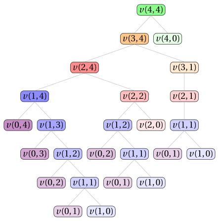
    The function \(v\) is called \(25\) times, and the same subproblems are solved multiple times: \(v(1,2)\) is called \(2\) times, \(v(0,2)\) is called \(2\) times, \(v(1,1)\) is called \(3\) times, \(v(0,1)\) is called \(3\) times, and \(v(1,0)\) is called \(3\) times. All the other calls are made only once.

  • The value \(v(j,\ell)\) can be computed once \(v(j-1,\ell)\) is known and, when \(j\le\ell\), \(v(j,\ell-j)\) is also known. Therefore, for a fixed value of \(j\), all values \(v(j,\ell)\) can be computed by considering the values of \(\ell\) in increasing order.

  • Starting from the base cases \(v(j,0)=0\) and \(v(0,\ell)=-\infty\), the values of the function \(v\) can be computed row by row, moving to the next value of \(j\) only after all values \(v(j,\ell)\) for the current value of \(j\) have been computed.

    Example 28.10: Computing the values of the \(v\) function

    We consider the RCP instance of Example 28.1 with a rod of length \(n = 4\) and the profits associated with the possible piece lengths are:

    \[ \begin{array}{l|rrrrrrr} \hline & {\ell = 1} & {\ell = 2} & {\ell = 3} & {\ell = 4} \\ \hline {p_\ell} & {1} & {5} & {8} & {9} \\ \hline \end{array} \]

    The values of the function \(v\) are computed as follows:

    • For \(j=1\), only pieces of length \(1\) can be used. Therefore:

      \[ v(1,0)=0, \]
      \[ v(1,1)=\max\{v(0,1),p_1+v(1,0)\}=\max\{-\infty,1+0\}=1, \]
      \[ v(1,2)=\max\{v(0,2),p_1+v(1,1)\}=\max\{-\infty,1+1\}=2, \]
      \[ v(1,3)=\max\{v(0,3),p_1+v(1,2)\}=\max\{-\infty,1+2\}=3, \]
      \[ v(1,4)=\max\{v(0,4),p_1+v(1,3)\}=\max\{-\infty,1+3\}=4. \]

    • For \(j=2\), pieces of length \(1\) and \(2\) can be used. We obtain:

      \[ v(2,0)=0,\qquad v(2,1)=v(1,1)=1, \]
      \[ v(2,2)=\max\{v(1,2),p_2+v(2,0)\}=\max\{2,5+0\}=5, \]
      \[ v(2,3)=\max\{v(1,3),p_2+v(2,1)\}=\max\{3,5+1\}=6, \]
      \[ v(2,4)=\max\{v(1,4),p_2+v(2,2)\}=\max\{4,5+5\}=10. \]

    • For \(j=3\), pieces of length \(1\), \(2\), and \(3\) can be used. We obtain:

      \[ v(3,0)=0,\qquad v(3,1)=v(2,1)=1,\qquad v(3,2)=v(2,2)=5, \]
      \[ v(3,3)=\max\{v(2,3),p_3+v(3,0)\}=\max\{6,8+0\}=8, \]
      \[ v(3,4)=\max\{v(2,4),p_3+v(3,1)\}=\max\{10,8+1\}=10. \]

    • For \(j=4\), all piece lengths are available. We obtain:

      \[ \begin{gathered} v(4,0)=0,\qquad v(4,1)=v(3,1)=1,\\ v(4,2)=v(3,2)=5,\qquad v(4,3)=v(3,3)=8, \end{gathered} \]
      \[ v(4,4)=\max\{v(3,4),p_4+v(4,0)\}=\max\{10,9+0\}=10. \]

  • We can avoid solving the same subproblems repeatedly by storing the value of each subproblem as soon as it is computed. The values are stored in a lookup table.

  • Since solving any particular subproblem depends only on subproblems with a smaller value of \(j\), or with the same value of \(j\) and a smaller rod length, we can solve the subproblems in increasing order of \(j\) and, for each fixed value of \(j\), in increasing order of rod length, starting from the base cases \(v(0,0)=0\) and \(v(0,\ell)=-\infty\) for all \(\ell \in \{1,\dots,n\}\) and building up to \(v(n,n)\).

  • This observation naturally leads to a much more efficient method to compute the optimal value \(v(n,n)\) of the RCP instance.

  • A second method to compute the optimal value \(v(n,n)\) of the RCP instance is the bottom-up approach. The method starts from the base cases \(v(0,0)=0\) and \(v(0,\ell)=-\infty\) for all \(\ell \in \{1,\dots,n\}\) and evaluates formula \(\eqref{eq:rcpalt}\) for increasing values of \(j \in \{1,2,\dots,n\}\) and \(\ell \in \{0,1,\dots,n\}\): each value \(v(j,\ell)\) is computed using already-computed values, until the value \(v(n,n)\) of the RCP instance is obtained.

    This is the pseudo-code of the DP algorithm using the bottom-up approach:

    Algorithm: DP2

    Input: An RCP instance given by the length \(n\) of the rod and an array \(p[1..n]\) of piece profits

    Output: The optimal value of the RCP instance

    1Function DP2(\(n,p\))

    2\({v} := \textnormal{new array}[0..n][0..n]\)

    3\({v}[0][0] \leftarrow 0\)

    4for \(\ell := 1\) to \(n\) do

    5\({v}[0][\ell] \leftarrow -\infty\)

    6end

    7for \(j := 1\) to \(n\) do

    8for \(\ell := 0\) to \(n\) do

    9if \(j > \ell\) then

    10\({v}[j][\ell] \leftarrow {v}[j-1][\ell]\)

    11else

    12if \(p[j] + {v}[j][\ell-j] > {v}[j-1][\ell]\) then

    13\({v}[j][\ell] \leftarrow p[j] + {v}[j][\ell-j]\)

    14else

    15\({v}[j][\ell] \leftarrow {v}[j-1][\ell]\)

    16end

    17end

    18end

    19end

    20return \({v}[n][n]\)

    • The matrix \({v}[0..n][0..n]\) is the lookup table: it stores the optimal values of all subproblems.

    • The initialization sets \({v}[0][0]=0\) and \({v}[0][\ell]=-\infty\) for all rod lengths \(\ell \in \{1,\dots,n\}\), since a positive length cannot be filled if no piece length is available.

    • The outer loop, over \(j \in \{1,2,\dots,n\}\), considers the available piece lengths in increasing order.

    • The inner loop, over \(\ell \in \{0,1,\dots,n\}\), computes the best value for each rod length using only pieces of length at most \(j\).

    • If \(j>\ell\), piece length \(j\) cannot be used, and therefore \({v}[j][\ell] \leftarrow {v}[j-1][\ell]\).

    • Otherwise, the DP algorithm compares the value obtained by not using piece length \(j\), namely \({v}[j-1][\ell]\), with the value obtained by using one piece of length \(j\), namely \(p[j]+{v}[j][\ell-j]\).

    • Finally, the optimal value of the RCP instance is returned as \({v}[n][n]\).

    Example 28.11: Execution of the DP algorithm

    We consider the RCP instance of Example 28.1 with a rod of length \(n = 4\) and the profits associated with the possible piece lengths are:

    \[ \begin{array}{l|rrrrrrr} \hline & {\ell = 1} & {\ell = 2} & {\ell = 3} & {\ell = 4} \\ \hline {p_\ell} & {1} & {5} & {8} & {9} \\ \hline \end{array} \]

    For each step of the DP algorithm, the table shows the values of \(j\) and \(\ell\), the cell \({v}[j][\ell]\), and the operation performed.

    \(j\)	\(\ell\)	\({v}[j][\ell]\)	Action
    \(0\)	\(0\)	0	\({v}[0][0]\leftarrow 0\)
    \(0\)	\(1\)	\(-\infty\)	\({v}[0][1]\leftarrow -\infty\)
    \(0\)	\(2\)	\(-\infty\)	\({v}[0][2]\leftarrow -\infty\)
    \(0\)	\(3\)	\(-\infty\)	\({v}[0][3]\leftarrow -\infty\)
    \(0\)	\(4\)	\(-\infty\)	\({v}[0][4]\leftarrow -\infty\)
    \(1\)	\(0\)	0	\({v}[1][0]\leftarrow {v}[0][0]=0\)
    \(1\)	\(1\)	1	\(\max\{{v}[0][1],p[1]+{v}[1][0]\}=\max\{-\infty,1+0\}=1\)
    \(1\)	\(2\)	2	\(\max\{{v}[0][2],p[1]+{v}[1][1]\}=\max\{-\infty,1+1\}=2\)
    \(1\)	\(3\)	3	\(\max\{{v}[0][3],p[1]+{v}[1][2]\}=\max\{-\infty,1+2\}=3\)
    \(1\)	\(4\)	4	\(\max\{{v}[0][4],p[1]+{v}[1][3]\}=\max\{-\infty,1+3\}=4\)
    \(2\)	\(0\)	0	\({v}[2][0]\leftarrow {v}[1][0]=0\)
    \(2\)	\(1\)	1	\(2>1\): \({v}[2][1]\leftarrow {v}[1][1]=1\)
    \(2\)	\(2\)	5	\(\max\{{v}[1][2],p[2]+{v}[2][0]\}=\max\{2,5+0\}=5\)
    \(2\)	\(3\)	6	\(\max\{{v}[1][3],p[2]+{v}[2][1]\}=\max\{3,5+1\}=6\)
    \(2\)	\(4\)	10	\(\max\{{v}[1][4],p[2]+{v}[2][2]\}=\max\{4,5+5\}=10\)
    \(3\)	\(0\)	0	\({v}[3][0]\leftarrow {v}[2][0]=0\)
    \(3\)	\(1\)	1	\(3>1\): \({v}[3][1]\leftarrow {v}[2][1]=1\)
    \(3\)	\(2\)	5	\(3>2\): \({v}[3][2]\leftarrow {v}[2][2]=5\)
    \(3\)	\(3\)	8	\(\max\{{v}[2][3],p[3]+{v}[3][0]\}=\max\{6,8+0\}=8\)
    \(3\)	\(4\)	10	\(\max\{{v}[2][4],p[3]+{v}[3][1]\}=\max\{10,8+1\}=10\)
    \(4\)	\(0\)	0	\({v}[4][0]\leftarrow {v}[3][0]=0\)
    \(4\)	\(1\)	1	\(4>1\): \({v}[4][1]\leftarrow {v}[3][1]=1\)
    \(4\)	\(2\)	5	\(4>2\): \({v}[4][2]\leftarrow {v}[3][2]=5\)
    \(4\)	\(3\)	8	\(4>3\): \({v}[4][3]\leftarrow {v}[3][3]=8\)
    \(4\)	\(4\)	10	\(\max\{{v}[3][4],p[4]+{v}[4][0]\}=\max\{10,9+0\}=10\)

    This is the matrix \({v}\) after the execution of the DP algorithm:

    \[ \begin{array}{l|rrrrr} \hline {{v}[j][\ell]} & {\ell=0} & {\ell=1} & {\ell=2} & {\ell=3} & {\ell=4} \\ \hline {j=0} & 0 & {-\infty} & {-\infty} & {-\infty} & {-\infty} \\ {j=1} & 0 & 1 & 2 & 3 & 4 \\ {j=2} & 0 & 1 & 5 & 6 & 10 \\ {j=3} & 0 & 1 & 5 & 8 & 10 \\ {j=4} & 0 & 1 & 5 & 8 & 10 \\ \hline \end{array} \]

  • After the execution of the DP algorithm, the matrix \({v}\) contains the optimal value \({v}[j][\ell]\) for every subproblem \((j,\ell)\).

• Step 2: computation of an optimal solution

  • To compute an optimal solution, it is necessary to store some additional information.

  • For each value \(j\) of the largest available piece length and each rod length \(\ell\), in addition to the optimal value \({v}[j][\ell]\), we store \({s}[j][\ell]\), which is equal to \(1\) if one piece of length \(j\) is used and to \(0\) otherwise.

  • Starting from \(j=n\) and \(\ell=n\), if \({s}[j][\ell]=0\), then piece length \(j\) is not used and \(j\) is decreased by \(1\). If \({s}[j][\ell]=1\), then one piece of length \(j\) is used and the residual rod length becomes \(\ell-j\). The procedure stops when the residual length reaches \(0\).

    This is the pseudo-code of the DP algorithm using the bottom-up approach with the storing of the information necessary to compute an optimal solution:

    Algorithm: DP2_InfoSol

    Input: An RCP instance given by the length \(n\) of the rod and an array \(p[1..n]\) of piece profits

    Output: The optimal value of the RCP instance and the matrix of binary information \({s}[0..n][0..n]\)

    1Function DP2_InfoSol(\(n,p\))

    2\({v} := \textnormal{new array}[0..n][0..n]\)

    3\({s} := \textnormal{new array}[0..n][0..n]\)

    4\({v}[0][0] \leftarrow 0\)

    5\({s}[0][0] \leftarrow 0\)

    6for \(\ell := 1\) to \(n\) do

    7\({v}[0][\ell] \leftarrow -\infty\)

    8\({s}[0][\ell] \leftarrow 0\)

    9end

    10for \(j := 1\) to \(n\) do

    11for \(\ell := 0\) to \(n\) do

    12if \(j > \ell\) then

    13\({v}[j][\ell] \leftarrow {v}[j-1][\ell]\)

    14\({s}[j][\ell] \leftarrow 0\)

    15else

    16if \(p[j] + {v}[j][\ell-j] > {v}[j-1][\ell]\) then

    17\({v}[j][\ell] \leftarrow p[j] + {v}[j][\ell-j]\)

    18\({s}[j][\ell] \leftarrow 1\)

    19else

    20\({v}[j][\ell] \leftarrow {v}[j-1][\ell]\)

    21\({s}[j][\ell] \leftarrow 0\)

    22end

    23end

    24end

    25end

    26return \({v}[n][n], {s}\)

    • The DP algorithm uses the additional matrix \({s}\), which keeps track of the decision made when \({v}[j][\ell]\) is computed. If one piece of length \(j\) is selected, \({s}[j][\ell]\leftarrow 1\) stores this decision; otherwise, \({s}[j][\ell]\leftarrow 0\) stores that piece length \(j\) is not used.

    Example 28.12: Computation of the additional information

    We consider the RCP instance of Example 28.1 with a rod of length \(n = 4\) and the profits associated with the possible piece lengths are:

    \[ \begin{array}{l|rrrrrrr} \hline & {\ell = 1} & {\ell = 2} & {\ell = 3} & {\ell = 4} \\ \hline {p_\ell} & {1} & {5} & {8} & {9} \\ \hline \end{array} \]

    For each step of the DP algorithm, the table shows the values of \(j\) and \(\ell\), the cell \({s}[j][\ell]\), and the operation performed.

    \(j\)	\(\ell\)	\({s}[j][\ell]\)	Action
    \(0\)	\(0\)	0	\({s}[0][0]\leftarrow 0\)
    \(0\)	\(1\)	0	\({s}[0][1]\leftarrow 0\)
    \(0\)	\(2\)	0	\({s}[0][2]\leftarrow 0\)
    \(0\)	\(3\)	0	\({s}[0][3]\leftarrow 0\)
    \(0\)	\(4\)	0	\({s}[0][4]\leftarrow 0\)
    \(1\)	\(0\)	0	\(1>0\): \({s}[1][0]\leftarrow 0\)
    \(1\)	\(1\)	1	\(p[1]+{v}[1][0]=1+0>{v}[0][1]=-\infty\): \({s}[1][1]\leftarrow 1\)
    \(1\)	\(2\)	1	\(p[1]+{v}[1][1]=1+1>{v}[0][2]=-\infty\): \({s}[1][2]\leftarrow 1\)
    \(1\)	\(3\)	1	\(p[1]+{v}[1][2]=1+2>{v}[0][3]=-\infty\): \({s}[1][3]\leftarrow 1\)
    \(1\)	\(4\)	1	\(p[1]+{v}[1][3]=1+3>{v}[0][4]=-\infty\): \({s}[1][4]\leftarrow 1\)
    \(2\)	\(0\)	0	\(2>0\): \({s}[2][0]\leftarrow 0\)
    \(2\)	\(1\)	0	\(2>1\): \({s}[2][1]\leftarrow 0\)
    \(2\)	\(2\)	1	\(p[2]+{v}[2][0]=5+0>{v}[1][2]=2\): \({s}[2][2]\leftarrow 1\)
    \(2\)	\(3\)	1	\(p[2]+{v}[2][1]=5+1>{v}[1][3]=3\): \({s}[2][3]\leftarrow 1\)
    \(2\)	\(4\)	1	\(p[2]+{v}[2][2]=5+5>{v}[1][4]=4\): \({s}[2][4]\leftarrow 1\)
    \(3\)	\(0\)	0	\(3>0\): \({s}[3][0]\leftarrow 0\)
    \(3\)	\(1\)	0	\(3>1\): \({s}[3][1]\leftarrow 0\)
    \(3\)	\(2\)	0	\(3>2\): \({s}[3][2]\leftarrow 0\)
    \(3\)	\(3\)	1	\(p[3]+{v}[3][0]=8+0>{v}[2][3]=6\): \({s}[3][3]\leftarrow 1\)
    \(3\)	\(4\)	0	\(p[3]+{v}[3][1]=8+1\le {v}[2][4]=10\): \({s}[3][4]\leftarrow 0\)
    \(4\)	\(0\)	0	\(4>0\): \({s}[4][0]\leftarrow 0\)
    \(4\)	\(1\)	0	\(4>1\): \({s}[4][1]\leftarrow 0\)
    \(4\)	\(2\)	0	\(4>2\): \({s}[4][2]\leftarrow 0\)
    \(4\)	\(3\)	0	\(4>3\): \({s}[4][3]\leftarrow 0\)
    \(4\)	\(4\)	0	\(p[4]+{v}[4][0]=9+0\le {v}[3][4]=10\): \({s}[4][4]\leftarrow 0\)

    This is the matrix \({s}\) after the execution of the DP algorithm:

    \[ \begin{array}{l|rrrrr} \hline {{s}[j][\ell]} & {\ell=0} & {\ell=1} & {\ell=2} & {\ell=3} & {\ell=4} \\ \hline {j=0} & 0 & 0 & 0 & 0 & 0 \\ {j=1} & 0 & 1 & 1 & 1 & 1 \\ {j=2} & 0 & 0 & 1 & 1 & 1 \\ {j=3} & 0 & 0 & 0 & 1 & 0 \\ {j=4} & 0 & 0 & 0 & 0 & 0 \\ \hline \end{array} \]

  • Once the matrix \({s}\) has been computed, an optimal solution for a rod of length \(n\) can be computed by repeatedly applying the following rule, starting from \((j,\ell)=(n,n)\) and \(x_h=0\) for all \(h \in \{1,2,\dots,n\}\):

    \[ \begin{array}{ll} j \leftarrow j-1 & \textrm{if ${s}[j][\ell]=0$,}\\[1ex] x_j \leftarrow x_j+1,\quad \ell \leftarrow \ell-j & \textrm{if ${s}[j][\ell]=1$.} \end{array} \]

    The procedure stops when \(\ell=0\). This yields the vector \((x_1,x_2,\dots,x_n)\), where each entry \(x_h\) is the number of pieces of length \(h\) in an optimal solution.

  • The following pseudo-code implements the computation of an optimal solution, given the matrix \({s}\).

    Algorithm: DP2_SolComputation

    Input: The rod length \(n\) and the matrix \({s}[0..n][0..n]\)

    Output: An optimal solution of the RCP instance

    1Function DP2_SolComputation(\(n,{s}\))

    2\(x := \textnormal{new array}[1..n]\)

    3for \(h := 1\) to \(n\) do

    4\(x[h] \leftarrow 0\)

    5end

    6\(j := n\)

    7\(\ell := n\)

    8while \(\ell > 0\) do

    9if \({s}[j][\ell] = 0\) then

    10\(j \leftarrow j-1\)

    11else

    12\(x[j] \leftarrow x[j]+1\)

    13\(\ell \leftarrow \ell-j\)

    14end

    15end

    16return \(x\)

    Example 28.13: Computing an optimal solution

    After the execution of the DP algorithm on the instance of Example 28.1, we have the following matrix \({s}\):

    \[ \begin{array}{l|rrrrr} \hline {{s}[j][\ell]} & {\ell=0} & {\ell=1} & {\ell=2} & {\ell=3} & {\ell=4} \\ \hline {j=0} & 0 & 0 & 0 & 0 & 0 \\ {j=1} & 0 & 1 & 1 & 1 & 1 \\ {j=2} & 0 & 0 & 1 & 1 & 1 \\ {j=3} & 0 & 0 & 0 & 1 & 0 \\ {j=4} & 0 & 0 & 0 & 0 & 0 \\ \hline \end{array} \]

    We can compute an optimal solution for a rod of length \(n=4\) as follows:

    Iteration	\(j\)	\(\ell\)	\({s}[j][\ell]\)	\(x[1]\)	\(x[2]\)	\(x[3]\)	\(x[4]\)	Action
    \(1\)	\(4\)	\(4\)	\(0\)	0	0	0	0	\(j\leftarrow 3\)
    \(2\)	\(3\)	\(4\)	\(0\)	0	0	0	0	\(j\leftarrow 2\)
    \(3\)	\(2\)	\(4\)	\(1\)	0	1	0	0	\(x[2]\leftarrow 1\), \(\ell\leftarrow 4-2=2\)
    \(4\)	\(2\)	\(2\)	\(1\)	0	2	0	0	\(x[2]\leftarrow 2\), \(\ell\leftarrow 2-2=0\)

    An optimal solution is the vector:

    \[ (0,2,0,0) \]

  • The same computation procedure, based on the matrix \({s}\), can be applied to any rod length \(\ell \le n\) by starting from \(j=n\).

    Example 28.14: Computing optimal solutions

    After the execution of the DP algorithm on the instance of Example 28.1, we have the following matrix \({s}\):

    \[ \begin{array}{l|rrrrr} \hline {{s}[j][\ell]} & {\ell=0} & {\ell=1} & {\ell=2} & {\ell=3} & {\ell=4} \\ \hline {j=0} & 0 & 0 & 0 & 0 & 0 \\ {j=1} & 0 & 1 & 1 & 1 & 1 \\ {j=2} & 0 & 0 & 1 & 1 & 1 \\ {j=3} & 0 & 0 & 0 & 1 & 0 \\ {j=4} & 0 & 0 & 0 & 0 & 0 \\ \hline \end{array} \]

    We can compute an optimal solution for a rod of length \(\ell=3\) as follows:

    Iteration	\(j\)	\(\ell\)	\({s}[j][\ell]\)	\(x[1]\)	\(x[2]\)	\(x[3]\)	\(x[4]\)	Action
    \(1\)	\(4\)	\(3\)	\(0\)	0	0	0	0	\(j\leftarrow 3\)
    \(2\)	\(3\)	\(3\)	\(1\)	0	0	1	0	\(x[3]\leftarrow 1\), \(\ell\leftarrow 3-3=0\)

    An optimal solution is the vector:

    \[ (0,0,1,0) \]

    We can compute an optimal solution for a rod of length \(\ell=2\) as follows:

    Iteration	\(j\)	\(\ell\)	\({s}[j][\ell]\)	\(x[1]\)	\(x[2]\)	\(x[3]\)	\(x[4]\)	Action
    \(1\)	\(4\)	\(2\)	\(0\)	0	0	0	0	\(j\leftarrow 3\)
    \(2\)	\(3\)	\(2\)	\(0\)	0	0	0	0	\(j\leftarrow 2\)
    \(3\)	\(2\)	\(2\)	\(1\)	0	1	0	0	\(x[2]\leftarrow 1\), \(\ell\leftarrow 2-2=0\)

    An optimal solution is the vector:

    \[ (0,1,0,0) \]

28.3.1 Number of steps

• Let \(S(n)\) denote the number of steps executed by DP2 in the worst case, where \(n\) is the rod length. We compute \(S(n)\) by counting how many times the lines of the pseudo-code of DP2 are executed.

• The number of times each line of code is executed is:

  • Line 2 is executed \(1\) time.

  • Line 3 is executed \(1\) time.

  • Line 4 is executed \(n\) times.

  • Line 5 is executed \(n\) times.

  • Line 7 is executed \(n\) times.

  • Line 8 is executed \(n(n+1)\) times.

  • Line 9 is executed \(n(n+1)\) times.

  • Line 12 is checked only when \(j\le \ell\), that is

    \[ \sum_{j=1}^{n}(n-j+1)=\sum_{j=1}^{n}j=\frac{n(n+1)}{2} \]

    times.

  • One among Line 10, Line 13, and Line 15 is executed for each pair \((j,\ell)\), and therefore these assignment lines are executed \(n(n+1)\) times in total.

  • Line 20 is executed \(1\) time.

  Therefore, the total number of steps in the worst case is

  \[ 1+1+n+n+n+n(n+1)+n(n+1)+\frac{n(n+1)}{2}+n(n+1)+1. \]

  Thus,

  \[ S(n)=3+3n+3n(n+1)+\frac{n(n+1)}{2} = \frac{7n^2+13n+6}{2}. \]

  Hence,

  \[ S(n)=\Theta(n^2). \]

  Indeed,

  \[ \lim_{n\to\infty} \frac{\frac{7n^2+13n+6}{2}}{n^2} = \lim_{n\to\infty} \frac{1}{2}\left(7+\frac{13}{n}+\frac{6}{n^2}\right) = \frac{7}{2}\in\mathbb{R}_{>0}. \]

  The DP algorithm executes

  \[ S(n)=\Theta(n^2) \]

  steps in the worst case.

---

Next: Typical mistakes · In summary