DP for the 0/1 knapsack problem
Part 3 · Dynamic programming · Chapter 17 · Lecture notes, volume 3 (PDF) · Slides (1/2) · Slides (2/2) · Exercises: 0/1 knapsack (KP) · App: DP tables for the knapsack problems
Prerequisites
-
From this module, the chapter «Principles of dynamic programming»: optimal substructure, overlapping subproblems, recurrence relations, base cases, and the top-down and bottom-up approaches.
-
From this module, the chapter «Knapsack problems»: the 0/1 knapsack problem (KP), the binary encoding of a solution, and the \(2^n\) subsets of items.
-
From the module Algorithms: how to read pseudocode (Chapter 2), and the size of the input of an algorithm (Chapter 11) (needed to explain why \(\Theta(nc)\) is pseudo-polynomial).
Where we were
-
As a problem: the KP, its instances and the \(2^n\) subsets (chapter «Knapsack problems»).
-
As a model: the ILP model, its LP relaxation and the dual bounds (chapter «Formulations of knapsack problems»).
-
Now, as a table: the DP algorithm computes the optimal value exactly, with no model and no solver.
Objectives
At the end of this chapter you will be able to:
-
write the recurrence \(v(j,k)\) of the KP, explain why it is correct, and compute the table by hand with the top-down approach, the bottom-up approach and a single vector;
-
reconstruct an optimal solution from the matrix \({s}\) of the decisions;
-
count the steps of the DP algorithm and explain why \(\Theta(nc)\) is pseudo-polynomial, not polynomial;
-
describe the states \((w,p)\), discard the dominated ones, and run the DP algorithm on lists of states;
-
exchange the roles of profits and weights, and compute the optimal value from the table \(u(j,q)\).
The problem of this chapter is the 0/1 knapsack problem (KP): its definition and its assumptions are on its page.
17.1 Instances and feasible solutions
Example 17.1: KP instance
We consider a knapsack of capacity \(c = 5\) and a set \(\{1,2,3\}\) of \(3\) items (\(n = 3\)), with the following profits and weights:
We refer to this KP instance as Example 17.1.
The number of possible subsets of items is \(2^n\) since, for each item, there is an independent option of inserting it or not into the knapsack. Some subsets may not respect the knapsack capacity. Accordingly, the number of feasible solutions is at most \(2^n\).
- The number of possible KP solutions grows exponentially with the number \(n\) of items. Therefore, enumerating all possible solutions quickly becomes impractical as \(n\) increases.
17.1.1 Encoding of feasible solutions
A feasible solution of the KP is a subset of items whose total weight does not exceed the knapsack capacity.
-
A KP feasible solution can be described by the binary vector
\[ (x_1,x_2,\dots,x_n) \]where each component has the following meaning:
\[ x_j = \left\{ \begin{array}{ll} 1 & \textrm{if item } j \textrm{ is selected,}\\[1ex] 0 & \textrm{otherwise,} \end{array} \right. \qquad \forall j \in \{1,2,\dots,n\}. \]Since the solution is feasible, the total weight of the selected items must not exceed the knapsack capacity:
\[ \sum_{j=1}^{n} w_j x_j \le c. \]The total profit of a feasible solution is
\[ \sum_{j=1}^{n} p_j x_j. \]
Example 17.2: Enumeration of all possible KP solutions
We consider the KP instance of Example 17.1 with a knapsack of capacity \(c=5\) and the following profits and weights:
There are \(2^3 = 8\) possible subsets of items, corresponding to the different ways of selecting or not selecting the items.
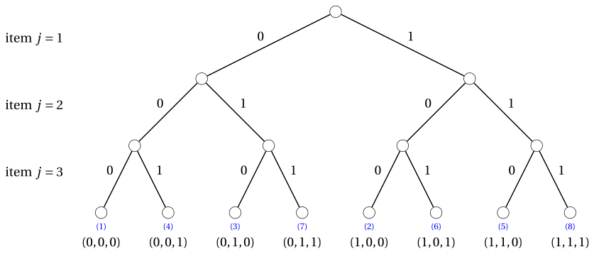
In the following binary tree, each level corresponds to an item: an edge labeled \(1\) means that the item is selected, while an edge labeled \(0\) means that it is not selected. Each leaf represents one complete subset of items and reports the corresponding vector.
The figure below shows the subsets associated with the leaves of the tree, through the labels \((1),(2),\ldots,(8)\). For each selected item, the number written inside the parallelepiped is its weight, while the number above it is its profit. The width of each parallelepiped is proportional to the item weight. Subsets whose total weight exceeds the knapsack capacity are marked as not feasible.
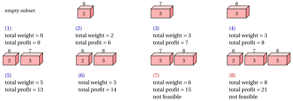
| Label | Solution vector | Total weight | Total profit | Feasible? |
|---|---|---|---|---|
| \((1)\) | \((0,0,0)\) | \(0\) | \(0\) | yes |
| \((2)\) | \((1,0,0)\) | \(2\) | \(6\) | yes |
| \((3)\) | \((0,1,0)\) | \(3\) | \(7\) | yes |
| \((4)\) | \((0,0,1)\) | \(3\) | \(8\) | yes |
| \((5)\) | \((1,1,0)\) | \(2+3=5\) | \(6+7=13\) | yes |
| \((6)\) | \((1,0,1)\) | \(2+3=5\) | \(6+8=14\) | yes |
| \((7)\) | \((0,1,1)\) | \(3+3=6\) | \(7+8=15\) | no |
| \((8)\) | \((1,1,1)\) | \(2+3+3=8\) | \(6+7+8=21\) | no |
-
Overview
Instances and feasible solutions · Encoding of feasible solutions
-
17.2 A first DP algorithm
-
17.2.2 A first DP algorithm: An implementation with lists
-
17.3 A second DP algorithm
-
17.3.2 A second DP algorithm: An implementation with lists
-
Typical mistakes · In summary
In summary
Next: 17.2 A first DP algorithm
Exercises on this chapter: 0/1 knapsack (KP)
In the interactive lab: DP tables for the knapsack problems.