Knapsack: branch-and-bound on the critical item¶

Part 6 · Ad hoc algorithms · Chapter 41 · Lecture notes, volume 6 (PDF) · Slides · Exercises: 0/1 knapsack (KP) · App: Branch-and-bound for the knapsack

Prerequisites

From the module Integer linear programming, Chapter 7 «Branch-and-bound»: branching and bounding operations, the problem list, the pruning criteria, the lower bound \(\LB\) and the upper bound \(\UB\). The general algorithm is applied here to the 0/1 knapsack problem.
From this module, Chapter 9 «Formulations of knapsack problems»: the models \(\mathrm{ILP}_{\mathrm{KP}}\) and \(\mathrm{LP}_{\mathrm{KP}}\), the efficiency of an item, the split item \(s\), the residual capacity \(\mathit{rc}\) and the bound of Dantzig.

Objectives

At the end of this chapter you will be able to:

write the problem \(\mathrm{LP}_{\mathrm{KP}}^k\) of a node, and solve it with the formulas of Dantzig, without the simplex algorithm;
branch on the variable of the split item, unselecting or selecting that item;
execute the branch-and-bound algorithm for the KP by hand, with the FIFO or the LIFO rule;
explain why the algorithm is simpler than the general one, and what stays the same.

The problem of this chapter is the 0/1 knapsack problem (KP): its definition and its assumptions are on its page.

41.1 The algorithm for the KP¶

Definition 41.1: branching node and \(\mathrm{LP}_{\mathrm{KP}}^k\) problem

In the branch-and-bound algorithm for the \(\mathrm{ILP}_{\mathrm{KP}}\) model, the branching constraints on a variable \(x_j\), \(j \in \mathscr{I}\), are \(x_j \le 0\) and \(x_j \ge 1\). In a branching node \(k\) of the branch-and-bound tree, we have:

a subset of unselected items \(\rightsquigarrow\) denoted \(\mathscr{I}_\text{out}^k\)
a subset of selected items \(\rightsquigarrow\) denoted \(\mathscr{I}_\text{in}^k\)
a subset of remaining items \(\rightsquigarrow\) denoted \(\mathscr{I}^k := \mathscr{I} \setminus \left\{\mathscr{I}^k_\text{out} \cup \mathscr{I}^k_\text{in} \right\}\)

The \(\mathrm{LP}_{\mathrm{KP}}\) problem associated to node \(k\), called the \(\mathrm{LP}_{\mathrm{KP}}^k\) problem, reads as follows:

\[\begin{align*} && \max \;\;{\sum_{j \in \mathscr{I}} p_j \, x_j} \\[1.5ex] && \text{subject to} \quad {\sum_{j \in \mathscr{I}} w_j \, x_j} &\leq c, \\[1.5ex] && x_j &\ge 1, & \forall j \in \mathscr{I}^k_\text{in},\\[1.5ex] && x_j &\le 0, & \forall j \in \mathscr{I}^k_\text{out},\\[1.5ex] && x_j &\le 1, & \forall j \in \mathscr{I},\\[1.5ex] &&x_j &\ge 0, & \forall j \in \mathscr{I}. \end{align*}\]

The branching constraints \(x_j \le 0\) and \(x_j \ge 1\) have the effect of unselecting or selecting an item.

A \(\mathrm{LP}_{\mathrm{KP}}^k\) problem of a branching node \(k\) can be equivalently re-written as:

\[\begin{align*} && \underbrace{ \sum_{j \in \mathscr{I}^k_\text{in} } p_j}_{=p(k)} + \max \;\;{\sum_{j \in \mathscr{I}^k } p_j \, x_j} \label{eq:KP-obj_LP} \tag{41.1a}\\[2ex] && \text{subject to} \quad {\sum_{j \in \mathscr{I}^k} w_j \, x_j} &\leq \underbrace{c - \sum_{j \in \mathscr{I}^k_\text{in} } w_j}_{=c(k)}, \label{eq:KP-cap_LP} \tag{41.1b}\\[2ex] && x_j &\le 1, & \forall j \in \mathscr{I}^k, \tag{41.1c}\\[2ex] && x_j &\ge 0, & \forall j \in \mathscr{I}^k. \label{eq:KP-bin_LP} \tag{41.1d} \end{align*}\]

A \(\mathrm{LP}^k_{\mathrm{KP}}\) problem of a branching node \(k\) is structurally equivalent to the \(\mathrm{LP}_{\mathrm{KP}}\) problem but:
1. the set of items is \(\mathscr{I}^k\) instead of \(\mathscr{I}\)
2. the capacity is reduced to \(c(k):=c - \sum_{j \in \mathscr{I}^k_\text{in} } w_j\)
3. there is an objective-function constant \(p(k):=\sum_{j \in \mathscr{I}^k_\text{in} } p_j\)

41.1.1 Solving the \(\mathrm{LP}_{\mathrm{KP}}^k\) problem of a node¶

The problem \(\mathrm{LP}_{\mathrm{KP}}^k\) is a knapsack LP problem on the items of \(\mathscr{I}^k\), with capacity \(c(k)\): it is solved by the formulas of Dantzig, without any simplex iteration. The items of \(\mathscr{I}^k\) are kept in the order of non-increasing efficiency.
If \(c(k)<0\) the problem is infeasible. If \(\sum_{j\in\mathscr{I}^k} w_j \le c(k)\) all the items of \(\mathscr{I}^k\) fit, and the optimal solution is \(\tilde{x}_j=1\) for all \(j\in\mathscr{I}^k\): it is integer.
Otherwise the split item \(s\) of the node, also called the critical item, is the first item of \(\mathscr{I}^k\) that does not fit entirely, and the residual capacity is the capacity left by the items that precede it:

\[ \sum_{j\in\mathscr{I}^k,\,j<s} w_j \le c(k) < \sum_{j\in\mathscr{I}^k,\,j\le s} w_j, \qquad \mathit{rc}=c(k)-\sum_{j\in\mathscr{I}^k,\,j<s} w_j . \]
The optimal solution is \(\tilde{x}_j=1\) for the items of \(\mathscr{I}^k\) before \(s\), \(\tilde{x}_s=\frac{\mathit{rc}}{w_s}\) and \(\tilde{x}_j=0\) for the items after \(s\), and the optimal value is

\[ z(\mathrm{LP}_{\mathrm{KP}}^k) \;=\; p(k)+\sum_{j\in\mathscr{I}^k,\,j<s} p_j + p_s\,\frac{\mathit{rc}}{w_s}. \]

In every node at most one variable is fractional, the one of the split item, and the value of the node is the Dantzig bound of a smaller knapsack: the node is solved by a scan of the items.

41.1.2 Branching-variable selection strategy¶

The optimal solution of an \(\mathrm{LP}_{\mathrm{KP}}^k\) problem given by the formulas of the previous subsection has at most one fractional variable, the one associated to the split item. Branching can be performed on the variable associated to the split item: this branching-variable selection strategy is called split-item strategy.
The optimal solution of an \(\mathrm{LP}_{\mathrm{KP}}\) problem is not unique when some items have equal efficiency: the other optimal solutions can have more fractional variables, for instance \(x=(\frac12,\frac12)\) for \(p=(2,2)\), \(w=(2,2)\), \(c=2\). Here, as in the general algorithm, we always use the solution given by the formulas.

41.1.3 What changes with respect to the general algorithm¶

The algorithm is the LP-based branch-and-bound algorithm of the module Integer linear programming (Chapter 7 «Branch-and-bound»), with its problem list, its pruning criteria and its optimality gap.
Bounding. The problem of a node is solved by the formulas above. All the profits are integer, so the bound of a node is \(\lfloor z(\mathrm{LP}_{\mathrm{KP}}^k)\rfloor\): the node is pruned by bound if \(\lfloor z(\mathrm{LP}_{\mathrm{KP}}^k)\rfloor \le \LB\), by infeasibility if \(c(k)<0\), by integrality if its solution is integer (then \(\LB\) is updated when the value is larger). An integer node is pruned by integrality even when its value does not exceed \(\LB\).
Branching. The branching variable is the one of the split item \(s\): the children are \(x_s\le 0\) (down, item unselected) and \(x_s\ge 1\) (up, item selected), and the node is not solved with a simplex tableau but described by the sets \(\mathscr{I}^k_\text{in}\), \(\mathscr{I}^k_\text{out}\) and \(\mathscr{I}^k\).
Node selection. The node of the problem list is extracted with the FIFO or the LIFO rule, and the down-branching node is solved before the up-branching node; the nodes are numbered in the order of resolution. The lower bound written in a node is the value at the moment of its resolution.

41.2 A worked example¶

Example 41.1: The \(\mathrm{ILP}_{\mathrm{KP}}\) model

We consider a knapsack of capacity \(c = 9\) and a set \(\mathscr{I} = \{1,2,3,4,5,6\}\) of \(6\) items (\(n = 6\)), with the following profits and weights:

\[ \begin{array}{l|rrrrrrr} \hline & {j = 1} & {j = 2} & {j = 3} & {j = 4} & {j = 5} & {j = 6} \\ \hline {p_j} & {6} & {5} & {8} & {9} & {6} & {7} \\ {w_j} & {2} & {3} & {6} & {7} & {5} & {9} \\ \hline \end{array} \]

We refer to this KP instance as Example 41.1. The \(\mathrm{ILP}_{\mathrm{KP}}\) model for this KP instance is:

\[ \begin{array}{rrrrrrrrrrrrr} {\max} & 6 \, {x_1} & + 5 \, {x_2} & + 8 \, {x_3} & + 9 \, {x_4} & + 6 \, {x_5} & + 7 \, {x_6} \\[0.5ex] \text{subject to} & 2 \, {x_1} & + 3 \, {x_2} & + 6 \, {x_3} & + 7 \, {x_4} & + 5 \, {x_5} & + 9 \, {x_6} & {\le} & 9 \\[0.5ex] & {x_1}, & {x_2}, & {x_3}, & {x_4}, & {x_5}, & {x_6} & { \in} & { \{0,1\}} \end{array} \]

An optimal solution \(~{\tilde{\vet x}}(\,\mathrm{ILP}_{\mathrm{KP}}\,)\) is:

\[ \tilde x_1=1,~~\tilde x_2=0,~~\tilde x_3=0,~~\tilde x_4=1,~~\tilde x_5=0,~~\tilde x_6=0 \]

The optimal value \(z(\mathrm{ILP}_{\mathrm{KP}})\) is \(15\). The associated optimal solution of the KP is \(\tilde{S} =\{1,4\}\).

The items are sorted by non-increasing efficiency, since:

\[ \frac{6}{2} ~~\ge~~ \frac{5}{3} ~~\ge~~ \frac{8}{6} ~~\ge~~ \frac{9}{7} ~~\ge~~ \frac{6}{5} ~~\ge~~ \frac{7}{9} \]

Example 41.2: Branch-and-bound algorithm for the \(\mathrm{ILP}_{\mathrm{KP}}\) model

A branch-and-bound algorithm for the \(\mathrm{ILP}_{\mathrm{KP}}\) model and the KP instance of Example 41.1 using:

the split-item strategy as branching-variable selection strategy;
the FIFO rule as branching-node selection strategy;
solve first the down-branching node and then the up-branching node;
set the incumbent solution \(\bar{\vet x}(\mathrm{ILP}_{\mathrm{KP}})\) to the following heuristic solution:

\[ \bar{x}_1=1, ~~~ \bar{x}_2=0,~~~ \bar{x}_3= 0,~~\bar{x}_4=1,~~\bar{x}_5=0,~~\bar{x}_6=0 \]

and set the lower bound \(\LB\) accordingly.
Initialization

For the \(\mathrm{LP}^1_{\mathrm{KP}}\) problem, the split item is \(s=3\) and the residual capacity is \(\mathit{rc} = 4\). An optimal solution \(\tilde{\vet x}(\,\mathrm{LP}^1_{\mathrm{KP}}\,)\) is:

\[ \tilde{x}_1=1,~~\tilde{x}_2=1,~~\tilde{x}_3=\frac{2}{3},~~\tilde{x}_4=0,~~\tilde{x}_5=0,~~\tilde{x}_6=0 \]

the optimal value is:

\[ z(~\mathrm{LP}^1_{\mathrm{KP}}~) = 6 \cdot 1 + 5 \cdot 1 + 8 \cdot \frac{2}{3} =\frac{49}{3} \]

The optimal solution \(\tilde{\vet x}(\,\mathrm{LP}^1_{\mathrm{KP}}\,)\) is fractional and the \(\mathrm{LP}^1_{\mathrm{KP}}\) problem is feasible, so the \(\mathrm{LP}^1_{\mathrm{KP}}\) problem is inserted in the problem list \(L\) and the lower bound \(\LB\) is set to \(15\) (\(\LB(\bar{\vet x})= 15\)).

Due to the current lower bound \(\LB\) and upper bound \(\UB\), we have:

\[ 15 ~~\le~~ z(\mathrm{ILP}_{\mathrm{KP}}) ~~\le~~ \underbrace{\left\lfloor \dfrac{49}{3} \right\rfloor}_{=16} \]
Iteration 1

The \(\mathrm{LP}^1_{\mathrm{KP}}\) problem is extracted and deleted from the problem list \(L\).

The branching variable is \(x_3\). The \(\mathrm{LP}^2_{\mathrm{KP}}\) and \(\mathrm{LP}^3_{\mathrm{KP}}\) problems are created by unselecting (\(x_3 \le 0\)) and selecting (\(x_3 \ge 1\)) item \(3\).
1. Solution of the \(\mathrm{LP}^2_{\mathrm{KP}}\) problem
  
  We have
  
  \[ \mathscr{I}^2 = \{1,2,4,5,6\},~~~\mathscr{I}^2_\text{out} = \{3\}, ~~~\mathscr{I}^2_\text{in} = \emptyset \]
  
  The capacity is \(c(2)=9\) and the objective-function constant is \(p(2)=0\). The split item is \(s=4\) and the residual capacity is \(\mathit{rc} = 4\). An optimal solution \(\tilde{\vet x}(\,\mathrm{LP}^2_{\mathrm{KP}}\,)\) is:
  
  \[ \tilde{x}_1=1,~~\tilde{x}_2=1,~~\tilde{x}_4=\frac{4}{7},~~\tilde{x}_5=0,~~\tilde{x}_6=0 \]
  
  and
  
  \[ z(~\mathrm{LP}^2_{\mathrm{KP}}~) = 6 \cdot 1 + 5 \cdot 1 + 9 \cdot \frac{4}{7} = \frac{113}{7} \]
  
  The \(\mathrm{LP}^2_{\mathrm{KP}}\) problem is feasible and we have:
  
  \[ \left\lfloor z(\mathrm{LP}^2_{\mathrm{KP}}) \right\rfloor > \LB \qquad \text{since} \qquad \underbrace{\left\lfloor\frac{113}{7} \right\rfloor}_{ = 16} >15 \]
  
  The optimal solution \(\tilde{\vet x}(\,\mathrm{LP}^2_{\mathrm{KP}}\,)\) is fractional, accordingly, the \(\mathrm{LP}^2_{\mathrm{KP}}\) problem is inserted in the problem list \(L\).
2. Solution of the \(\mathrm{LP}^3_{\mathrm{KP}}\) problem
  
  We have
  
  \[ \mathscr{I}^3 = \{1,2,4,5,6\},~~~\mathscr{I}^3_\text{out} = \emptyset, ~~~\mathscr{I}^3_\text{in} = \{3\} \]
  
  The capacity is \(c(3)=3\) and the objective-function constant is \(p(3)=8\). The split item is \(s=2\) and the residual capacity is \(\mathit{rc} = 1\). An optimal solution \(\tilde{\vet x}(\,\mathrm{LP}^3_{\mathrm{KP}}\,)\) is:
  
  \[ \tilde{x}_1=1,~~\tilde{x}_2=\frac{1}{3},~~\tilde{x}_4=0,~~\tilde{x}_5=0,~~\tilde{x}_6=0 \text{ and } z(~\mathrm{LP}^3_{\mathrm{KP}}~) = 8 + 6 \cdot 1 + 5 \cdot \frac{1}{3} = \frac{47}{3} \]
  
  The \(\mathrm{LP}^3_{\mathrm{KP}}\) problem is feasible and we have:
  
  \[ \left\lfloor z(\mathrm{LP}^3_{\mathrm{KP}}) \right\rfloor \le \LB \qquad \text{since} \qquad \underbrace{\left\lfloor\frac{47}{3} \right\rfloor}_{ = 15} \le 15 \]
  
  accordingly, the branching node is pruned by upper bound.
At the end of the first iteration, Node 2 is inserted in the problem list \(L\), while Node 3 is pruned by upper bound. The corresponding branch-and-bound tree is:

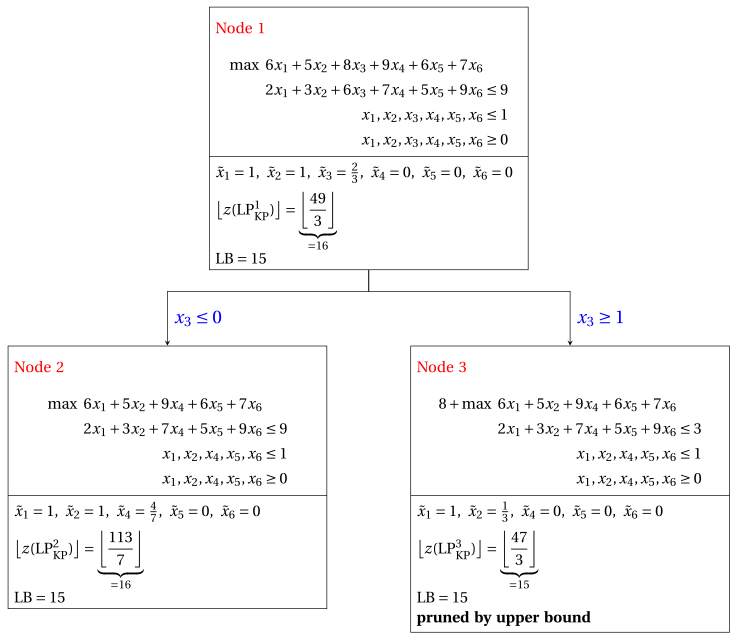
Due to the current lower bound \(\LB\) and upper bound \(\UB\), we have:

\[ 15 ~~\le~~ z(\mathrm{ILP}_{\mathrm{KP}}) ~~\le~~ \underbrace{\left\lfloor \dfrac{113}{7} \right\rfloor}_{=16} \]
Iteration 2

The \(\mathrm{LP}^2_{\mathrm{KP}}\) problem is extracted and deleted from the problem list \(L\).

The branching variable is \(x_4\). The \(\mathrm{LP}^4_{\mathrm{KP}}\) and \(\mathrm{LP}^5_{\mathrm{KP}}\) problems are created by unselecting (\(x_4 \le 0\)) and selecting (\(x_4 \ge 1\)) item \(4\).
1. Solution of the \(\mathrm{LP}^4_{\mathrm{KP}}\) problem
  
  We have
  
  \[ \mathscr{I}^4 = \{1,2,5,6\},~~~\mathscr{I}^4_\text{out} = \{3,4\}, ~~~\mathscr{I}^4_\text{in} = \emptyset \]
  
  The capacity is \(c(4)=9\) and the objective-function constant is \(p(4)=0\). The split item is \(s=5\) and the residual capacity is \(\mathit{rc} = 4\). An optimal solution \(\tilde{\vet x}(\,\mathrm{LP}^4_{\mathrm{KP}}\,)\) is:
  
  \[ \tilde{x}_1=1,~~\tilde{x}_2=1,~~\tilde{x}_5=\frac{4}{5},~~\tilde{x}_6=0 \text{ and } z(~\mathrm{LP}^4_{\mathrm{KP}}~) = 6 \cdot 1 + 5 \cdot 1 + 6 \cdot \frac{4}{5} = \frac{79}{5} \]
  
  The \(\mathrm{LP}^4_{\mathrm{KP}}\) problem is feasible and we have:
  
  \[ \left\lfloor z(\mathrm{LP}^4_{\mathrm{KP}}) \right\rfloor \le \LB \qquad \text{since} \qquad \underbrace{\left\lfloor\frac{79}{5} \right\rfloor}_{ = 15} \le 15 \]
  
  accordingly, the branching node is pruned by upper bound.
2. Solution of the \(\mathrm{LP}^5_{\mathrm{KP}}\) problem
  
  We have
  
  \[ \mathscr{I}^5 = \{1,2,5,6\},~~~\mathscr{I}^5_\text{out} = \{3\}, ~~~\mathscr{I}^5_\text{in}= \{4\} \]
  
  The capacity is \(c(5)=2\) and the objective-function constant is \(p(5)=9\). The split item is \(s=2\) and the residual capacity is \(\mathit{rc} = 0\). An optimal solution \(\tilde{\vet x}(\,\mathrm{LP}^5_{\mathrm{KP}}\,)\) is:
  
  \[ \tilde{x}_1=1,~~\tilde{x}_2=0,~~\tilde{x}_5=0,~~\tilde{x}_6=0 \text{ and } z(~\mathrm{LP}^5_{\mathrm{KP}}~) = 9 + 6 \cdot 1 = 15 \]
  
  The \(\mathrm{LP}^5_{\mathrm{KP}}\) problem is feasible and its optimal solution \(\tilde{\vet x}(\,\mathrm{LP}^5_{\mathrm{KP}}\,)\) is integer. Its value does not improve the incumbent solution, since \(z(\mathrm{LP}^5_{\mathrm{KP}})=15 \le 15=\LB\), so the lower bound \(\LB\) stays \(15\). Accordingly, the branching node is pruned by integrality: when a node could be pruned both by integrality and by bound, it is pruned by integrality.
At the end of the second iteration, Node 4 is pruned by upper bound and Node 5 is pruned by integrality. The corresponding branch-and-bound tree is:
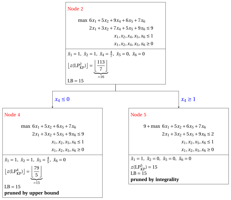
Termination

Since the problem list \(L\) is empty, the \(\mathrm{ILP}_{\mathrm{KP}}\) problem is solved to optimality.

The optimal value is \(z(\mathrm{ILP}_{\mathrm{KP}})=15\) (the value of the lower bound \(\LB\)) and an optimal solution \(\tilde{\vet x}(\,\mathrm{ILP}_{\mathrm{KP}}\,)\) is \(\tilde x_1=1,\tilde x_2=0,\tilde x_3=0,\tilde x_4=1,\tilde x_5=0,\tilde x_6=0\) (the incumbent solution \(\bar{\vet x}(\mathrm{ILP}_{\mathrm{KP}})\)).

This is the branch-and-bound tree of the previous execution of the branch-and-bound algorithm, showing for each branching node the optimal value of the associated \(\mathrm{LP}_{\mathrm{KP}}\) problem, the lower bound \(\LB\), and the pruning criteria.

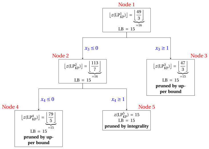
41.3 Typical mistakes¶

Warning

Forgetting the upper bounds \(x_j\le 1\). Without them the LP problem of a node would put all the capacity on the item of best efficiency: the node boxes must contain \(x_j\le 1\).
Computing the split item on the original instance. In a node, the split item and the residual capacity are computed on the items of \(\mathscr{I}^k\) with the capacity \(c(k)\), after fixing the items of \(\mathscr{I}^k_\text{in}\) and \(\mathscr{I}^k_\text{out}\).
Forgetting the constant \(p(k)\). The value of the node is \(p(k)\) plus the value of the items of \(\mathscr{I}^k\): the profit of the selected items counts.
Using the old lower bound. The lower bound is updated as soon as a node has an integer solution of larger value; the nodes of the list that become dominated are discarded.
Numbering the skipped children. A child that is not solved does not receive a node index, exactly as in the general algorithm.

41.4 In summary¶

In summary

The branch-and-bound algorithm for the KP is the LP-based algorithm with two simplifications: the problem of every node is solved by the formulas of Dantzig, and the branching variable is the one of the split item.
A node is described by the sets \(\mathscr{I}^k_\text{in}\), \(\mathscr{I}^k_\text{out}\) and \(\mathscr{I}^k\), by the capacity \(c(k)\) and by the constant \(p(k)\).
The bound of a node is \(\lfloor z(\mathrm{LP}_{\mathrm{KP}}^k)\rfloor\); when the problem list is empty the lower and the upper bound coincide and the incumbent solution is optimal.

Dashboard of the KP instance of Example 41.1 (\(c=9\), \(p=(6,5,8,9,6,7)\), \(w=(2,3,6,7,5,9)\)). The bounds on \(z(\mathrm{ILP}_{\mathrm{KP}})\) found so far:

Source	Lower bound	Upper bound	From
Dantzig bound	–	\(16\)	\(\left\lfloor \frac{49}{3} \right\rfloor\)
This chapter, initialization	\(15\)	\(16\)	heuristic solution \(\{1,4\}\)
This chapter, iteration \(1\)	\(15\)	\(16\)	node \(2\) in the list, \(\left\lfloor \frac{113}{7} \right\rfloor\)
This chapter, termination	\(15\)	\(15\)	empty list, \(5\) nodes

Exercises on this chapter: 0/1 knapsack (KP)

In the interactive lab: Branch-and-bound for the knapsack.