32.2 The problems and the assumptions
Part 4 · Heuristic algorithms · Chapter 32 · Chapter 32: Metaheuristics · Lecture notes, volume 4 (PDF) · Slides (1/2) · Slides (2/2) · Exercises: Metaheuristics · App: TSP: simulated annealing and tabu search
- The metaheuristics are illustrated on the four problems of the chapter «Heuristic algorithms: definitions»: the 0/1 knapsack problem (KP), the bin packing problem (BPP), the travelling salesman problem (TSP) and \(P\,||\,C_{\max}\). Their definitions and assumptions are on their pages; we recall the notation.
| problem | data | solution | objective |
|---|---|---|---|
| KP | items \(\mathscr{I}\), profits \(p_j\), weights \(w_j\), capacity \(c\) | subset of items | max total profit |
| BPP | items \(\mathscr{I}\), weights \(w_j\), capacity \(c\) | patterns \(P_b\) | min number of bins |
| TSP | cities \(\mathscr{V}\), distances \(d_{ij}\) | tour \(\sigma\) | min length \(L(\sigma)\) |
| \(P\,||\,C_{\max}\) | jobs \(\mathscr{J}\), times \(t_j\), machines \(m\) | sets \(J_1,\dots,J_m\) | min makespan |
-
Every instance satisfies the assumptions of its problem: \(w_j\le c\) for all items and \(\sum_j w_j > c\) for the KP and the BPP; \(n\ge 3\) and symmetric distances for the TSP; \(n>m\) for \(P\,||\,C_{\max}\). For \(P\,||\,C_{\max}\), \(L_h=\sum_{j\in J_h}t_j\) is the load of machine \(h\) and \(C_{\max}=\max_h L_h\).
-
As in the chapter «Heuristic algorithms: definitions», \(\mathscr{A}(I)\) is the value of the solution computed by the algorithm \(\mathscr{A}\) on the instance \(I\), and \(z(I)\) is the optimal value. We write \(f(S)\) for the value of a solution \(S\), and we describe the algorithms for a minimization problem; for the KP, a maximization problem, the inequalities are reversed.
32.2.1 The neighbourhoods
- All the metaheuristics of this chapter are built on the neighbourhoods of the chapter «Local search». We recall them by name, with the moves that define them; \(n\) is the number of items, cities or jobs.
| problem | name | move | size |
|---|---|---|---|
| KP | flip | add one item to the knapsack, or remove one | \(n\) |
| swap | remove one selected item and add one unselected item | \(\le \frac{n^2}{4}\) | |
| BPP | move | move one item to another bin | \(\le n\cdot nb\) |
| swap | exchange two items packed in different bins | \(\le \frac{n(n-1)}{2}\) | |
| TSP | 2-opt | remove two non-adjacent edges of the tour and reconnect it with the two other edges, reversing the segment between them | \(\frac{n(n-3)}{2}\) |
| Or-opt | move a segment of \(1\), \(2\) or \(3\) consecutive cities to another position | \(O(n^2)\) | |
| \(P\,||\,C_{\max}\) | move | move one job to another machine | \(n(m-1)\) |
| swap | exchange two jobs assigned to different machines | \(\le \frac{n(n-1)}{2}\) |
-
A TSP tour is stored as a permutation \(\sigma=(\sigma_1,\dots,\sigma_n)\) with \(\sigma_1=1\). The 2-opt move \((i,j)\), with \(1\le i\), \(i+2\le j\le n\) and \((i,j)\neq(1,n)\), removes the edges \((\sigma_i,\sigma_{i+1})\) and \((\sigma_j,\sigma_{j+1})\) (with \(\sigma_{n+1}=\sigma_1\)), adds the edges \((\sigma_i,\sigma_j)\) and \((\sigma_{i+1},\sigma_{j+1})\), and reverses the segment \(\sigma_{i+1},\dots,\sigma_j\). Its effect on the length is computed in \(O(1)\):
\[ \delta(i,j) \;=\; d_{\sigma_i\sigma_j} + d_{\sigma_{i+1}\sigma_{j+1}} - d_{\sigma_i\sigma_{i+1}} - d_{\sigma_j\sigma_{j+1}} . \] -
The objectives of the BPP and of \(P\,||\,C_{\max}\) are flat: most moves do not change the number of bins, or the makespan. Two solutions with the same value are then compared with an auxiliary objective:
-
BPP: the sum of the squared loads \(\sum_b \big(\sum_{j\in P_b} w_j\big)^2\), to be maximized: it grows when the items concentrate in fewer, fuller bins;
-
\(P\,||\,C_{\max}\): the sum of the squared loads \(\sum_h L_h^2\), to be minimized: it decreases when the loads become balanced.
For \(P\,||\,C_{\max}\) we compare two solutions lexicographically: first by \(C_{\max}\), and if the makespans are equal, by \(\sum_h L_h^2\). For move and swap this selects the same improving moves as the auxiliary objective \(\sum_h L_h^2\) of the chapter «Local search»: a transfer that decreases \(\sum_h L_h^2\) never increases \(C_{\max}\), and a transfer that decreases \(C_{\max}\) also decreases \(\sum_h L_h^2\).
-
-
For the KP the flip neighbourhood contains infeasible solutions (adding an item may exceed the capacity). A local search either discards them or accepts them with a penalty on the excess weight; both options appear in this chapter.
-
The local searches used inside the metaheuristics are the descents of the chapter «Local search»: TWOOPTLS (2-opt, best improvement) for the TSP, MOVEDESCENT (move, best improvement, lexicographic comparison) for \(P\,||\,C_{\max}\), and KPLOCALSEARCH (feasible flips and swaps, best improvement) for the KP. In every best-improvement descent, ties between equally good moves are broken in favour of the first move found, scanning the indices in increasing order.
32.2.2 Random numbers
- Most metaheuristics make random choices. To make every example and every exercise reproducible, all the random numbers of this chapter, and of the code in the Colab notebooks of the chapter, are produced by the minimal standard generator of Park and Miller (1988):
A call \(\textsc{Rand}()\) updates \(seed\) and returns \(u\). A random integer in \(\{0,1,\dots,K-1\}\) is \(\lfloor u\cdot K\rfloor\), and a random element of a list of \(K\) elements is the element in position \(1+\lfloor u\cdot K\rfloor\).
-
The initial value of \(seed\), the seed, is an integer in \(\{1,\dots,2^{31}-2\}\). The same seed always gives the same sequence of numbers; different seeds give different runs of the same algorithm. With \(seed=1\) the first numbers are, rounded to four decimals,
\[ 0.0000,\ 0.1315,\ 0.7556,\ 0.4587,\ 0.5328,\ 0.2190,\ 0.0470,\ 0.6789,\ \dots \]The first number produced from a small seed is always very close to \(0\); it is a property of the generator, not an error.
-
In the worked examples the random numbers are written in the text, rounded to four decimals, so that every step can be checked by hand; the rounding never changes a decision.
32.2.3 The instances
- The worked examples use the four reference instances of the chapter «Heuristic algorithms: definitions», whose optimal values are known:
| problem | reference instance | optimal value and solution |
|---|---|---|
| KP | \(p=(10,7,6,4)\), \(w=(5,4,3,3)\), \(c=9\) | \(z(I)=17\), items \(\{1,2\}\) |
| BPP | \(w=(4,4,5,3,2,3)\), \(c=7\) | \(z(I)=3\), patterns \(\{1,4\},\{2,6\},\{3,5\}\) |
| TSP | \(5\) cities, distances \(d_{ij}\) below | \(z(I)=18\), tour \((1,3,5,2,4)\) |
| \(P\,||\,C_{\max}\) | \(t=(5,5,4,4,3,3,3)\), \(m=3\) | \(z(I)=9\), sets \(\{1,3\},\{2,4\},\{5,6,7\}\) |
- The reference instances are small enough to follow every iteration by hand, but too small to show the behaviour of a metaheuristic over thousands of iterations. For the experiments we use one medium instance per problem, generated once with the random number generator of Section 32.2.2 and fixed below. Their optimal values have been computed with an exact algorithm, and are used only to measure the quality of the heuristic solutions.
Example 32.1: The medium TSP instance (TSP20)
\(20\) cities in the plane, with integer coordinates \((x_i,y_i)\), and distances \(d_{ij}=\big\lfloor \sqrt{(x_i-x_j)^2+(y_i-y_j)^2} + \frac{1}{2}\big\rfloor\) (the Euclidean distance rounded to the nearest integer):
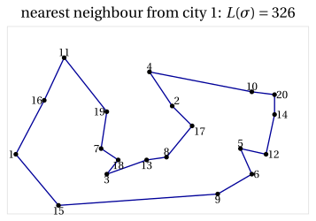
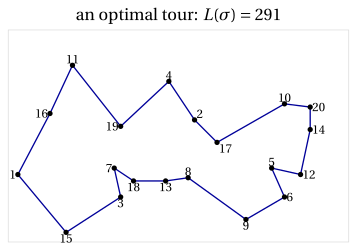
The nearest neighbour tour from city \(1\) has length \(326\); the 2-opt local search started from it stops at a local optimum of length \(319\), after two improving moves. The optimal value is \(z(I)=291\): the local optimum is \(9.6\%\) above it.
Example 32.2: The medium instances of the KP, the BPP and \(P\,||\,C_{\max}\)
KP20: \(n=20\) items, capacity \(c=389\) (half of the total weight, rounded down),
The greedy algorithm by efficiency finds profit \(490\), and the local search with flips and swaps started from it reaches \(514\); the optimal value is \(z(I)=521\).
PCM15: \(m=4\) machines and \(n=15\) jobs with processing times
The total time is \(275\), so \(z(I)\ge\lceil 275/4\rceil=69\), and an assignment of makespan \(69\) exists: \(z(I)=69\). LPT finds makespan \(73\).
BPP24: bins of capacity \(c=100\) and \(n=24\) items with weights
The total weight is \(868\), so at least \(\lceil 868/100\rceil=9\) bins are needed, and a packing into \(9\) bins exists: \(z(I)=9\). FF and FFD both use \(10\) bins.
Next: How to escape from a local optimum · Simulated annealing