MIP heuristics for the classical problems
Part 4 · Heuristic algorithms · Chapter 33 · Lecture notes, volume 4 (PDF) · Slides · Exercises: MIP heuristics
Prerequisites
-
From the module Integer Linear Programming, Chapter 10 «MIP heuristics»: the methods of this chapter (rounding, diving, the feasibility pump, RINS, local branching, proximity search, relax-and-fix and fix-and-optimize), their pseudo-codes and the conditions under which they work.
-
From this module, the chapters on the formulations of the classical problems (part «Formulations and their properties»): the models of the 0/1 knapsack problem, of the bin packing problem, of the travelling salesman problem, of \(P\,||\,C_{\max}\) and of lot sizing.
-
From this module, the chapters on heuristic algorithms, from «Heuristic algorithms: definitions» to «Metaheuristics»: the constructive heuristics (\(GR\), \(FF\), \(NN\), \(LPT\)), local search and metaheuristics, whose solutions are the starting points of this chapter.
Objectives
At the end of this chapter you will be able to:
-
write the MIP models of the classical problems in the form required by the MIP-based heuristics, and compute their LP relaxations;
-
execute by hand rounding, diving, the feasibility pump, RINS, local branching and proximity search on the 0/1 knapsack problem, on bin packing and on \(P\,||\,C_{\max}\);
-
execute relax-and-fix and fix-and-optimize on a lot sizing instance;
-
explain why each method succeeds or fails on each problem;
-
compute the gap of a heuristic solution when a dual bound is available.
33.1 MIP-based heuristics
Definition 33.1: MIP-based heuristic
A heuristic algorithm for a problem with a MIP model is MIP-based (a matheuristic) if it uses the LP relaxation of the model and a MIP solver to search for a feasible solution.
-
The MIP-based heuristics are defined in the module Integer Linear Programming, Chapter 10 «MIP heuristics». In this chapter they are applied to the classical problems, with the reference instances of the previous chapters.
-
The notation is that of that chapter: a MIP with integer variables \(\mathscr{D}\), \(\tilde{\vet x}\) is an optimal solution of the LP relaxation, \(\bar{\vet x}\) a feasible solution (the incumbent), \(\rnd{v}=\lfloor v+\frac12\rfloor\) the rounding to the nearest integer, \(\Delta(\vet x,\bar{\vet x})=\sum_{j\in\mathscr{D}}|x_j-\bar x_j|\) the distance from an integer point. A maximization problem, such as the KP, is handled by exchanging \(\min\) and \(\max\), \(\le\) and \(\ge\) in the comparisons of objective values.
-
The examples are solved with the MIP solver Gurobi, used from Python through
gurobipy. When an LP has several optimal solutions, the text reports the one returned by the solver; the codes are in the last section.
Constructive heuristics, local search and metaheuristics work on a representation of the solutions; a MIP-based heuristic works on the model of the problem, through its LP relaxation and a MIP solver.
33.2 The problems and their MIP models
-
The heuristics are illustrated on the four problems of the previous chapters: the 0/1 knapsack problem (KP), the bin packing problem (BPP), the travelling salesman problem (TSP) and \(P\,||\,C_{\max}\). Their definitions and assumptions are on their pages.
-
The reference instances are recalled in the following table, with the values computed in the previous chapters on heuristic algorithms.
| problem | reference instance | values |
|---|---|---|
| KP | \(p=(10,7,6,4)\), \(w=(5,4,3,3)\), \(c=9\) | \(GR\): \(\{1,3\}\), profit \(16\); \(z(I)=17\), \(\{1,2\}\) |
| BPP | \(w=(4,4,5,3,2,3)\), \(c=7\) | \(FF\): \(4\) bins; \(z(I)=3\) |
| TSP | \(5\) cities, the reference distances | \(NN\) from city \(1\): \(25\); \(z(I)=18\) |
| \(P\,||\,C_{\max}\) | \(t=(5,5,4,4,3,3,3)\), \(m=3\) | \(LPT\): \(J_1=\{1,5,7\}\), \(J_2=\{2,6\}\), \(J_3=\{3,4\}\), \(11\); \(z(I)=9\) |
- The MIP models are those of the part «Formulations and their properties»: the \(\mathrm{ILP}_{\mathrm{KP}}\) model of the chapter «Formulations of knapsack problems», the \(\mathrm{ILP}_{\mathrm{BPP}}\) model of the chapter «Formulations of packing problems», the \(\mathrm{ILP}_{\mathrm{TSP}}^{\mathrm{DFJ}}\) model of the chapter «Formulations of routing problems» and the \(\mathrm{ILP}_{P\|C_{\max}}\) model of the chapter «Formulations of scheduling problems». We recall the three models used in the examples, with the variables and the notation of those chapters.
33.2.1 The 0/1 knapsack problem
- The binary variable \(x_j\) is equal to \(1\) if item \(j\) is selected in the knapsack, and to \(0\) otherwise, for every \(j \in \mathscr{I}\).
Using these variables, an ILP model for the 0/1 knapsack problem (KP) reads as follows:
This ILP model is referred to as the \(\mathrm{ILP}_{\mathrm{KP}}\) model.
33.2.2 The bin packing problem
- Given an upper bound \(m\) on the number of bins used in an optimal solution, and the set \(\mathscr{B}=\{1,2,\dots,m\}\) of the available bins, the binary variable \(x_{jb}\) is equal to \(1\) if item \(j\) is packed in bin \(b\), and the binary variable \(y_b\) is equal to \(1\) if bin \(b\) is used, for every \(j\in\mathscr{I}\) and \(b\in\mathscr{B}\).
Using these variables, an ILP model for the bin packing problem (BPP) reads as follows:
This ILP model is referred to as the \(\mathrm{ILP}_{\mathrm{BPP}}\) model.
- The content of bin \(b\) is the packing pattern \(P_b=\{j\in\mathscr{I}: x_{jb}=1\}\). The number \(n\) of items is always a valid upper bound \(m\); on the reference instance we use \(m=n=6\).
33.2.3 The travelling salesman problem
- The \(\mathrm{ILP}_{\mathrm{TSP}}^{\mathrm{DFJ}}\) model has a binary variable \(x_{ij}\) for every arc \((i,j)\in A\), the constraints on the arcs leaving and entering every city, and the subtour elimination constraints on the subsets \(S\subseteq\mathscr{V}\setminus\{1\}\) with \(|S|\ge2\). On the reference instance, with \(n=5\) cities, it has \(20\) variables and \(5+5+11=21\) constraints.
33.2.4 The scheduling problem \(P\,||\,C_{\max}\)
- Given the set \(\mathscr{H}=\{1,2,\dots,m\}\) of the machines, the binary variable \(x_{jh}\) is equal to \(1\) if job \(j\) is assigned to machine \(h\), for every \(j\in\mathscr{J}\) and \(h\in\mathscr{H}\), and the non-negative continuous variable \(C_{\max}\) is the makespan.
Using these variables, an ILP model for \(P\|C_{\max}\) reads as follows:
This ILP model is referred to as the \(\mathrm{ILP}_{P\|C_{\max}}\) model.
- \(C_{\max}\) is the only continuous variable of the four models: given the assignment, the completion sets it to the largest load \(L_h=\sum_{j\in\mathscr{J}} t_j\,x_{jh}\).
33.2.5 The LP relaxations on the reference instances
- The following table reports the size of the four models on the reference instances, the value \(z(\mathrm{LP})\) of their LP relaxations, computed with Gurobi, and the optimal value \(z(I)\).
| problem | variables | constraints | \(z(\mathrm{LP})\) | \(z(I)\) | LP solution integer? |
|---|---|---|---|---|---|
| KP | \(4\) | \(1\) | \(17.75\) | \(17\) | no |
| BPP | \(42\) | \(12\) | \(3\) | \(3\) | no |
| TSP | \(20\) | \(21\) | \(18\) | \(18\) | yes |
| \(P\,||\,C_{\max}\) | \(22\) | \(10\) | \(9\) | \(9\) | no |
-
On all four instances the LP value, rounded in the direction of the bound (down for the KP, up for the three minimization problems), is already the optimal value. The relaxations are strong on these instances: the difficulty is to find a solution that attains the bound, not to prove it.
-
This is the typical situation in which MIP-based heuristics are useful.
-
On the TSP reference instance the LP solution of the \(\mathrm{ILP}_{\mathrm{TSP}}^{\mathrm{DFJ}}\) model is itself the optimal tour \((1,3,5,2,4)\), with \(\tilde x_{13}=\tilde x_{35}=\tilde x_{52}=\tilde x_{24}=\tilde x_{41}=1\): every method of this chapter finds it at once. The LP relaxation of the \(\mathrm{ILP}_{\mathrm{TSP}}^{\mathrm{MTZ}}\) model is weaker: its value is \(17\). The TSP is therefore not used in the other examples of this chapter.
Example 33.1: The LP solutions of the reference instances
KP. The LP solution is \(\tilde{\vet x}=\big(1,\frac14,1,0\big)\): the items are taken by non-increasing efficiency, and the split item \(2\) is taken for the fraction \(\frac{9-8}{4}=\frac14\) of its weight, so \(z(\mathrm{LP})=10+\frac74+6=17.75\).
\(P\,||\,C_{\max}\). The LP solution returned by the solver is (zeros omitted)
with loads \(L_1=3+5\cdot\frac35+3=9\), \(L_2=4\cdot\frac12+4+3=9\), \(L_3=5+5\cdot\frac25+4\cdot\frac12=9\) and \(\tilde C_{\max}=9=\frac{27}{3}\). The LP has infinitely many optimal solutions: every fractional assignment with three loads equal to \(9\) is optimal.
BPP. The LP solution returned by the solver puts item \(1\) into bin \(6\), item \(2\) into bin \(4\), item \(3\) for \(\frac45\) into bin \(3\) and for \(\frac15\) into bin \(4\), item \(4\) into bin \(6\), item \(5\) into bin \(1\), item \(6\) into bin \(3\), and opens the bins by the fractions
just enough to contain their loads: \(2\), \(0\), \(7\), \(5\), \(0\), \(7\). Its value is \(\frac{21}{7}=3\).
33.3 Rounding
- Rounding rounds the LP solution to the nearest integer point and completes the continuous variables; it fails if the rounded point violates a constraint. Rounding down is always feasible when all the coefficients of \(A\) are non-negative and \(b\ge0\) (the observation on rounding down of Chapter 10 «MIP heuristics» of the module Integer Linear Programming); an equality constraint, such as the assignment constraints of the BPP and of \(P\,||\,C_{\max}\), is almost always violated by independent roundings.
Example 33.2: Rounding on the reference instances
KP. The LP solution \(\tilde{\vet x}=\big(1,\frac14,1,0\big)\) is rounded to \(\bar{\vet x}=(1,0,1,0)\): weight \(8\le9\), profit \(16\). It is the solution of \(GR\) of the chapter «Constructive heuristics». Rounding \(\tilde x_2=\frac14\) up instead would give \((1,1,1,0)\), of weight \(12>9\): infeasible.
\(P\,||\,C_{\max}\). In the LP solution of Example 33.1, \(\rnd{\frac35}=1\) and \(\rnd{\frac25}=0\) send job \(2\) to machine \(1\), but \(\rnd{\frac12}=1\) assigns job \(3\) to both machines \(2\) and \(3\):
The assignment constraint \(\eqref{eq:pcm-assign}\) of job \(3\) is violated: rounding fails.
BPP. Rounding the LP solution of Example 33.1 gives \(\bar{\vet y}=(0,0,1,1,0,1)\) and puts item \(3\) into bin \(3\). Two capacity constraints \(\eqref{eq:bpp-cap}\) are violated: bin \(1\) contains item \(5\) but \(\bar y_1=0\) (\(-2+7\cdot 0\ge 0\) is false), and bin \(3\) contains items \(3\) and \(6\) (\(-(5+3)+7\cdot 1\ge 0\) is false). Rounding fails.
- The three outcomes summarize the method: on the KP, with a single packing constraint, rounding is safe (the observation on rounding down of Chapter 10 «MIP heuristics» of the module Integer Linear Programming); on the problems with assignment constraints it fails, because the LP spreads a job or an item over several machines or bins, and rounding cannot decide where it goes.
33.4 Diving
- Diving fixes one fractional variable at a time and re-solves the LP: fractional diving fixes the least fractional variable to its nearest integer, guided diving fixes the variable closest to the incumbent to the incumbent value; it fails when the LP becomes infeasible. Ties are broken in favour of the variable that comes first in the order of the variables (\(x_{11},x_{12},\dots\) for the assignment models, then \(C_{\max}\) or \(y_1,y_2,\dots\)).
Example 33.3: Fractional diving on the KP
Step 1. The LP solution is \(\tilde{\vet x}=\big(1,\frac14,1,0\big)\), of value \(17.75\). The only fractional variable is \(x_2\), rounded to \(\rnd{\frac14}=0\): fix \(x_2:=0\).
Step 2. Without item \(2\), the LP takes items \(1\) and \(3\) (weight \(8\)) and the fraction \(\frac13\) of item \(4\): \(\tilde{\vet x}=\big(1,0,1,\frac13\big)\), of value \(10+6+\frac43=\frac{52}{3}\approx 17.33\). Fix \(x_4:=\rnd{\frac13}=0\).
Step 3. The LP solution \(\tilde{\vet x}=(1,0,1,0)\), of value \(16\), is integer: the dive returns \(\{1,3\}\), of profit \(16\).
The dive is the path drawn with solid lines in the branch-and-bound tree below; the dashed nodes are the branches it never visits, with the value of their LP relaxations.
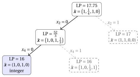
The branch \(x_2=1\), abandoned at the first step, contains the optimal solution \(\{1,2\}\) of profit \(17\), which is an optimal solution of its LP relaxation. The first decision of the dive, \(\rnd{\frac14}=0\), was the wrong one.
Example 33.4: Fractional diving on \(P\,||\,C_{\max}\)
The dive starts from the LP solution of Example 33.1. The table reports, for each step, the value of the LP, its fractional variables and the fixing; a fractionality \(|\tilde x_j-\rnd{\tilde x_j}|\) equal for two variables is broken by the order \(x_{11},x_{12},x_{13},x_{21},\dots\)
| step | LP value | fractional variables | fixing |
|---|---|---|---|
| \(1\) | \(9\) | \(x_{21}=\frac35\), \(x_{23}=\frac25\), \(x_{32}=\frac12\), \(x_{33}=\frac12\) | \(x_{21}:=1\) |
| \(2\) | \(9\) | \(x_{11}=\frac15\), \(x_{13}=\frac45\), \(x_{32}=\frac34\), \(x_{33}=\frac14\) | \(x_{11}:=0\) |
| \(3\) | \(9\) | \(x_{32}=\frac34\), \(x_{33}=\frac14\), \(x_{41}=\frac14\), \(x_{43}=\frac34\) | \(x_{32}:=1\) |
| \(4\) | \(9\) | \(x_{41}=\frac14\), \(x_{43}=\frac34\), \(x_{52}=\frac23\), \(x_{53}=\frac13\) | \(x_{41}:=0\) |
| \(5\) | \(9\) | \(x_{61}=\frac13\), \(x_{62}=\frac23\) | \(x_{61}:=0\) |
| \(6\) | \(9\) | \(x_{12}=\frac35\), \(x_{13}=\frac25\), \(x_{71}=\frac13\), \(x_{72}=\frac23\) | \(x_{71}:=0\) |
| \(7\) | \(9.5\) | \(x_{42}=\frac18\), \(x_{43}=\frac78\) | \(x_{42}:=0\) |
| \(8\) | \(9.5\) | \(x_{62}=\frac16\), \(x_{63}=\frac56\) | \(x_{62}:=0\) |
| \(9\) | \(9.5\) | \(x_{12}=\frac12\), \(x_{13}=\frac12\) | \(x_{12}:=1\) |
| \(10\) | \(9.5\) | \(x_{72}=\frac16\), \(x_{73}=\frac56\) | \(x_{72}:=0\) |
| \(11\) | \(10\) | none | — |
The last LP solution is integer: \(J_1=\{2,5\}\), \(J_2=\{1,3\}\), \(J_3=\{4,6,7\}\), with loads \(8\), \(9\), \(10\) and makespan \(10\). The dive improves on rounding, which failed, and on \(LPT\) (\(11\)), but it does not reach the optimum \(9\).
- For six steps the LP value stays at \(9\): the LP of \(P\,||\,C_{\max}\) has a huge set of optimal solutions, and fixing one variable just moves the LP to another of them. The LP value tells nothing about the quality of the decisions until the load of a machine is forced above \(9\), at step \(7\), and then it is too late to undo the decisions that caused it. Min-max objectives are as flat for the LP as they are for local search.
Example 33.5: Guided diving on \(P\,||\,C_{\max}\)
The incumbent is the solution of \(LPT\), \(J_1=\{1,5,7\}\), \(J_2=\{2,6\}\), \(J_3=\{3,4\}\), of makespan \(11\), i.e., \(\bar x_{11}=\bar x_{51}=\bar x_{71}=\bar x_{22}=\bar x_{62}=\bar x_{33}=\bar x_{43}=1\) and all the other \(\bar x_{jh}=0\).
Step 1. In the LP solution of Example 33.1 the fractional variables and their distances from the incumbent are
The closest is \(x_{23}\): fix \(x_{23}:=\bar x_{23}=0\).
Step 2. The new LP solution, of value \(9\), has the fractional variables \(x_{12}=\frac25\), \(x_{13}=\frac35\), \(x_{31}=\frac12\), \(x_{32}=\frac12\), at distances \(\frac25\), \(\frac35\), \(\frac12\), \(\frac12\) from the incumbent. Fix \(x_{12}:=\bar x_{12}=0\).
Step 3. The LP solution is integer, of value \(9\): \(J_1=\{5,6,7\}\), \(J_2=\{2,4\}\), \(J_3=\{1,3\}\), all loads equal to \(9\). Guided diving finds an optimal solution after two LPs.
-
Guided by a solution of makespan \(11\), the dive ends at a solution of makespan \(9\): the incumbent only decides the values of the two fixed variables, both equal to \(0\), while the LP rebuilds the rest of the assignment.
-
On the BPP reference instance, fractional diving takes \(8\) fixings, all with LP value \(3\); the ninth, \(x_{12}:=1\), puts item \(1\) into bin \(2\), which already contains item \(2\) by an earlier fixing, and \(4+4>7\) makes the LP infeasible: the dive fails. The fixings \(x_{jb}=1\) commit items to bins one at a time, and the LP of the BPP is so weak (\(3\) at every step) that it gives no warning before the dead end.
33.5 The feasibility pump
- The feasibility pump alternates the projection of an integer point onto the LP feasible region (one LP minimizing \(\Delta\)) and the rounding of the projection, with a flip when the rounding returns the same integer point and a random restart when the pump cycles, until the distance is \(0\). The random numbers are those of the minimal standard generator of Park and Miller with the seeds \(1,2,\dots\), as in the chapter «Metaheuristics».
Example 33.6: The feasibility pump on \(P\,||\,C_{\max}\)
Iteration 0. The LP solution of Example 33.1 is rounded as in Example 33.2: job \(3\) is assigned to machines \(2\) and \(3\), and \(\bar{\vet x}^0\) is infeasible.
Iteration 1. The projection minimizes \(\Delta(\vet x,\bar{\vet x}^0)\), which is linear since all the integer variables are binary. The solver returns the point of \(\mathcal{L}\) that keeps all the assignments of \(\bar{\vet x}^0\) and removes job \(3\) from machine \(2\), i.e., it moves \(x_{32}\) from \(1\) to \(0\): \(\Delta=1\) (removing job \(3\) from machine \(3\) would be equally close). The result is integer:
with loads \(11\), \(7\), \(9\), and its rounding is the new integer point \(\bar{\vet x}^1\).
Iteration 2. \(\bar{\vet x}^1\in\mathcal{L}\), the distance is \(0\), and the pump returns a solution of makespan \(11\), after two projections.
- The solution has the same makespan as \(LPT\): the projection takes care of the assignment constraints and ignores the loads, since \(C_{\max}\) is continuous and does not enter \(\Delta\). The pump answers the question “is there a feasible solution?”, which for \(P\,||\,C_{\max}\) was not a difficult question.
Example 33.7: The feasibility pump on the BPP
On the BPP reference instance, where rounding and diving fail, the pump is run with the seeds \(1,2,\dots,10\) of the random numbers. The table reports the number of projections, of flips and of restarts, the number of bins opened by the solution found (\(\sum_b \bar y_b\), the value of the solution) and the number of non-empty bins.
| seed | \(1\) | \(2\) | \(3\) | \(4\) | \(5\) | \(6\) | \(7\) | \(8\) | \(9\) | \(10\) |
|---|---|---|---|---|---|---|---|---|---|---|
| projections | \(15\) | \(12\) | \(9\) | \(9\) | \(6\) | \(6\) | \(19\) | \(5\) | \(10\) | \(20\) |
| flips | \(8\) | \(5\) | \(3\) | \(4\) | \(3\) | \(3\) | \(8\) | \(2\) | \(5\) | \(8\) |
| restarts | \(4\) | \(3\) | \(3\) | \(2\) | \(1\) | \(1\) | \(5\) | \(1\) | \(2\) | \(4\) |
| bins opened | \(4\) | \(4\) | \(4\) | \(5\) | \(5\) | \(4\) | \(3\) | \(4\) | \(4\) | \(5\) |
| non-empty bins | \(4\) | \(4\) | \(4\) | \(3\) | \(5\) | \(4\) | \(3\) | \(4\) | \(4\) | \(4\) |
The pump finds a feasible solution with every seed, but always after some restarts: without them it would cycle. Only with seed \(7\) the solution is optimal: \(\{3,5\}\), \(\{2,4\}\), \(\{1,6\}\), of value \(3\). With seed \(4\) the pump opens \(5\) bins, two of which stay empty: the packing \(\{3,5\}\), \(\{1,6\}\), \(\{2,4\}\) is optimal, but the solution has value \(5\), because nothing in the distance function asks to close the empty bins.
- The pump is a method to find a first feasible solution, and it does that well. The quality of the solution is the job of the improvement methods, which start from an incumbent.
33.6 RINS, local branching and proximity search
- The three methods start from an incumbent \(\bar{\vet x}\) and solve a sub-MIP with the cutoff constraint \(f(\vet x)\le f(\bar{\vet x})-\theta\), which here has \(\theta=1\) since the objective values are integer: RINS fixes the integer variables on which the LP solution and the incumbent agree; local branching adds \(\Delta(\vet x,\bar{\vet x})\le k\) and enlarges \(k\) when it finds nothing; proximity search minimizes \(\Delta(\vet x,\bar{\vet x})\).
33.6.1 RINS
Example 33.8: RINS on the KP
The incumbent is the solution \(\bar{\vet x}=(1,0,1,0)\) of \(GR\), of profit \(16\), and the LP solution is \(\tilde{\vet x}=\big(1,\frac14,1,0\big)\). They agree on \(x_1=1\), \(x_3=1\), \(x_4=0\), which are fixed. The sub-MIP, with the capacity constraint \(\eqref{eq:kp-cap}\) and the cutoff constraint, is
and it is infeasible: the capacity requires \(x_2=0\), the cutoff \(x_2=1\). RINS returns the incumbent. The optimal solution \(\{1,2\}\) has \(x_3=0\), but \(x_3\) is fixed to \(1\) because the LP and the incumbent agree on it.
Example 33.9: RINS on \(P\,||\,C_{\max}\)
The incumbent is the solution of \(LPT\) (\(J_1=\{1,5,7\}\), \(J_2=\{2,6\}\), \(J_3=\{3,4\}\), makespan \(11\)), and \(\tilde{\vet x}\) is the LP solution of Example 33.1. The table compares, for each job, the machine of the incumbent with the LP solution.
| \(j=1\) | \(j=2\) | \(j=3\) | \(j=4\) | \(j=5\) | \(j=6\) | \(j=7\) | |
|---|---|---|---|---|---|---|---|
| machine in \(\bar{\vet x}\) | \(1\) | \(2\) | \(3\) | \(3\) | \(1\) | \(2\) | \(1\) |
| machines in \(\tilde{\vet x}\) | \(3\) | \(1\) (\(\frac35\)), \(3\) (\(\frac25\)) | \(2\) (\(\frac12\)), \(3\) (\(\frac12\)) | \(2\) | \(2\) | \(1\) | \(1\) |
| fixed variables | \(x_{12}=0\) | — | \(x_{31}=0\) | \(x_{41}=0\) | \(x_{53}=0\) | \(x_{63}=0\) | \(x_{71}=1\), \(x_{72}=x_{73}=0\) |
Only job \(7\) is on the same machine in both solutions; for the other jobs, the two solutions agree only on some machines that the job does not use. Eight of the \(21\) binary variables are fixed. The sub-MIP with the cutoff \(C_{\max}\le 10\) is solved by Gurobi, which returns
with all loads equal to \(9\): RINS finds an optimal solution.
- On the KP the incumbent and the LP solution are too similar, and the neighbourhood of RINS has a single free variable; on \(P\,||\,C_{\max}\) they are very different, and the neighbourhood is large enough to contain the optimum.
33.6.2 Local branching
- Local branching and local search. With \(k=1\) the neighbourhood is the flip neighbourhood of the KP in the chapter «Heuristic algorithms: definitions»; with \(k=2\) it contains the swap neighbourhood as well. For the assignment variables of the BPP and of \(P\,||\,C_{\max}\) the distance has a simple meaning.
Observation 33.2
Let \(\vet x\) and \(\bar{\vet x}\) be two feasible assignments of \(P\,||\,C_{\max}\). Then \(\Delta(\vet x,\bar{\vet x})=2\,r\), where \(r\) is the number of jobs assigned to different machines in \(\vet x\) and in \(\bar{\vet x}\).
Proof
A job on the same machine in \(\vet x\) and \(\bar{\vet x}\) contributes \(0\) to \(\Delta\). A job on machine \(h\) in \(\bar{\vet x}\) and on machine \(h'\neq h\) in \(\vet x\) contributes \(1-x_{jh}=1\) and \(x_{jh'}=1\), and \(0\) for the other machines. □
- Hence, for \(P\,||\,C_{\max}\), the neighbourhood \(\Delta(\vet x,\bar{\vet x})\le 2\) is the move neighbourhood of the chapter «Local search» (one job changes machine), and \(\Delta(\vet x,\bar{\vet x})\le 4\) contains the swap neighbourhood (two jobs change machine). The same holds for the variables \(x_{jb}\) of the BPP.
Example 33.10: Local branching on the KP
Start from \(\bar{\vet x}^1=(1,0,1,0)\), of profit \(16\), with \(k=1\), \(k_{\max}=3\), \(k_{step}=1\) and \(\theta=1\).
\(k=1\). The neighbours at distance \(1\) are the flips of \(\bar{\vet x}^1\); with the cutoff \(\sum_j p_j x_j\ge 17\) no one is feasible. Add \(\Delta(\vet x,\bar{\vet x}^1)\ge 2\) and set \(k=2\).
\(k=2\). The sub-MIP with \(2\le\Delta(\vet x,\bar{\vet x}^1)\le 2\) finds the swap \((1,1,0,0)\), of profit \(17\): the new incumbent \(\bar{\vet x}^2\). Add \(\Delta(\vet x,\bar{\vet x}^1)\ge 3\).
\(k=2\), around \(\bar{\vet x}^2\). No solution of profit at least \(18\): add \(\Delta(\vet x,\bar{\vet x}^2)\ge 3\) and set \(k=3\). \(k=3\). No solution of profit at least \(18\) either; \(k\) becomes \(4>k_{\max}\) and the method stops with \(\{1,2\}\), of profit \(17\): the optimum.
Example 33.11: Local branching on \(P\,||\,C_{\max}\)
Start from the solution \(\bar{\vet x}^1\) of \(LPT\), of makespan \(11\), with \(k=2\), \(k_{\max}=6\), \(k_{step}=2\) and \(\theta=1\), so that the cutoff is \(C_{\max}\le 10\), then \(9\), and so on.
\(k=2\). By Observation 33.2 the neighbourhood is the move neighbourhood, and \(LPT\) is a local optimum for it (chapter «Local search»): the sub-MIP is infeasible. Add \(\Delta(\vet x,\bar{\vet x}^1)\ge 3\) and set \(k=4\).
\(k=4\). The best solution with two jobs reassigned has makespan \(10\); the solver returns the swap of jobs \(1\) and \(4\), \(\bar{\vet x}^2\) below. Add \(\Delta(\vet x,\bar{\vet x}^1)\ge 5\).
\(k=4\), around \(\bar{\vet x}^2\). The solver returns the swap of jobs \(4\) and \(6\), of makespan \(9\): \(\bar{\vet x}^3\). Add \(\Delta(\vet x,\bar{\vet x}^2)\ge 5\).
\(k=4\) and \(k=6\), around \(\bar{\vet x}^3\). No solution of makespan \(8\): \(k\) becomes \(8>k_{\max}\), and the method stops with makespan \(9\), the optimum.
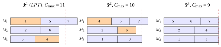
The dashed line is the lower bound \(9\); the jobs swapped to obtain the next solution are coloured.
- In the language of the chapter «Local search», local branching performs a local search with a neighbourhood whose size is controlled by \(k\), explored exactly by the solver, and it enlarges the neighbourhood when it gets stuck — exactly the idea of variable neighbourhood search, with the solver doing the exploration.
33.6.3 Proximity search
- A proximity sub-MIP that is infeasible with \(\theta=1\) proves that the incumbent is optimal, when the objective takes integer values (the proposition of Chapter 10 «MIP heuristics» of the module Integer Linear Programming).
Example 33.12: Proximity search on the KP
From \(\bar{\vet x}=(1,0,1,0)\), of profit \(16\): the closest solution of profit at least \(17\) is \((1,1,0,0)\), at distance \(2\) (item \(3\) out, item \(2\) in), of profit \(17\). Around it, no solution has profit at least \(18\): by the optimality condition of proximity search (Chapter 10 «MIP heuristics» of the module Integer Linear Programming), \(\{1,2\}\) is optimal.
Example 33.13: Proximity search on \(P\,||\,C_{\max}\)
From the solution of \(LPT\), of makespan \(11\):
| iteration | cutoff | \(\min\Delta\) | solution returned | \(C_{\max}\) |
|---|---|---|---|---|
| \(1\) | \(C_{\max}\le 10\) | \(4\) | \(J_1=\{5,6,7\}\), \(J_2=\{1,2\}\), \(J_3=\{3,4\}\) | \(10\) |
| \(2\) | \(C_{\max}\le 9\) | \(4\) | \(J_1=\{5,6,7\}\), \(J_2=\{1,4\}\), \(J_3=\{2,3\}\) | \(9\) |
| \(3\) | \(C_{\max}\le 8\) | — | infeasible | — |
By Observation 33.2, distance \(4\) means two jobs reassigned: jobs \(1\) and \(6\) at the first iteration, jobs \(2\) and \(4\) at the second. No solution at distance \(2\) improves the makespan, as for local branching with \(k=2\). At the third iteration the sub-MIP is infeasible, and the optimality condition of proximity search (Chapter 10 «MIP heuristics» of the module Integer Linear Programming) proves that makespan \(9\) is optimal.
- The proof of optimality comes from the solver, which proves the infeasibility of the last sub-MIP with its own dual bounds: proximity search, used with \(\theta=1\), is an exact method that improves the incumbent along the way.
33.7 Relax-and-fix and fix-and-optimize on lot sizing
-
Relax-and-fix and fix-and-optimize decompose the MIP into blocks of integer variables. Lot sizing is a natural application, because its variables are indexed by the periods \(t\in T=\{1,2,\dots,m\}\) of a planning horizon, and the decisions of a period mainly interact with those of the nearby periods. The blocks are the setup variables of consecutive periods.
-
The model is the \(\mathrm{ILP}_{\mathrm{CLSP}}\) model of the chapter «Formulations of lot sizing problems», with the strong big-M value \(M_t=\min\{cap_t,\,D_{t,m}\}\), where \(D_{t,m}=\sum_{k=t}^{m} d_k\); for an uncapacitated instance, \(cap_t=D_{t,m}\). Its variables are the production \(x_t\), the inventory \(s_t\) at the end of period \(t\) and the setup \(y_t\), for every period \(t\in T\).
Using these variables, an ILP model for the capacitated lot sizing problem (CLS) reads as follows:
This ILP model is referred to as the \(\mathrm{ILP}_{\mathrm{CLSP}}\) model.
-
Once the setups \(y\) are fixed, the rest is an LP with integer data and a network matrix, which has an integer optimal solution. The hard decisions are the \(m\) binary variables: as in the codes, the heuristics treat \(x_t\) and \(s_t\) as continuous variables, with \(x_t\ge 0\) and \(s_t\ge 0\) in place of \(\eqref{eq:ls-domx}\) and \(\eqref{eq:ls-doms}\).
-
The LP relaxation is weak, because a fraction \(y_t=x_t/M_t\) of a setup is enough to produce \(x_t\).
Example 33.14: Relax-and-fix on an uncapacitated lot sizing instance
The instance of the module MIP Modelling, Chapter 4 «Constructive heuristics», has \(m=5\) periods, \(d=(20,10,30,40,10)\), \(sc_t=50\), \(vc_t=0\) and \(hc_t=1\) for every \(t\in T\), and no capacity. Its LP relaxation has value \(\frac{36985}{396}\approx 93.40\), the constructive heuristic least unit cost of that chapter gives \(200\), and the optimal value is \(170\). Relax-and-fix with one period per block, \(B_t=\{y_t\}\), finds a solution of value \(170\): optimal.
Example 33.15: Relax-and-fix on a capacitated instance
Consider \(m=6\) periods, \(d=(50,30,10,10,40,10)\), \(sc_t=40\), \(vc_t=0\), \(hc_t=1\) and \(cap_t=80\) for every \(t\in T\). The LP relaxation has value \(\frac{2150}{21}\approx 102.38\) and the optimal value is \(160\), with setups in periods \(1\), \(2\), \(5\). Relax-and-fix with \(B_t=\{y_t\}\):
| step \(r\) | value of the MIP of step \(r\) | \(y\) of the solution | fixing |
|---|---|---|---|
| \(1\) | \(\frac{2465}{21}\approx 117.38\) | \(\big(1,\,0.375,\,0.143,\,0.167,\,1,\,0\big)\) | \(y_1:=1\) |
| \(2\) | \(\frac{2780}{21}\approx 132.38\) | \(\big(1,\,0,\,0.143,\,0.167,\,1,\,0\big)\) | \(y_2:=0\) |
| \(3\) | \(\frac{500}{3}\approx 166.67\) | \(\big(1,\,0,\,1,\,0.167,\,1,\,0\big)\) | \(y_3:=1\) |
| \(4\) | \(170\) | \((1,0,1,0,1,0)\) | \(y_4:=0\) |
| \(5\) | \(170\) | \((1,0,1,0,1,0)\) | \(y_5:=1\) |
| \(6\) | \(170\) | \((1,0,1,0,1,0)\) | \(y_6:=0\) |
(the fractional values are rounded to three decimals). The result has setups in periods \(1\), \(3\), \(5\): production \(80\), \(20\), \(50\), stocks \(30\), \(10\), \(10\) at the end of periods \(1\), \(3\), \(5\), cost \(3\cdot 40+50=170\). The wrong decision is taken at step \(2\): with the future relaxed, \(y_2=0\) gives \(132.38\) and \(y_2=1\) gives \(142.38\), so relax-and-fix saves the setup of period \(2\); but then the capacity forces a setup in period \(3\), which the relaxation had paid only for a fraction \(0.143\).
Example 33.16: Fix-and-optimize on the capacitated instance
Start from the solution of relax-and-fix of Example 33.15, \(\bar{\vet y}=(1,0,1,0,1,0)\) of cost \(170\), with the windows of two consecutive periods \(W_t=\{y_t,y_{t+1}\}\), \(t=1,2,\dots,5\).
| window | incumbent after the window | |
|---|---|---|
| \(\{y_1,y_2\}\) | \(170\) | no improvement |
| \(\{y_2,y_3\}\) | \(160\) | \(\bar{\vet y}=(1,1,0,0,1,0)\) |
| \(\{y_3,y_4\}\), \(\{y_4,y_5\}\), \(\{y_5,y_6\}\) | \(160\) | no improvement |
| second pass, all windows | \(160\) | no improvement: stop |
The window \(\{y_2,y_3\}\) revises the wrong decision of relax-and-fix: the setup moves from period \(3\) to period \(2\). The plan produces \(50\), \(50\), \(50\) in periods \(1\), \(2\), \(5\), with stocks \(20\) and \(10\) at the end of periods \(2\), \(3\) and \(10\) at the end of period \(5\): cost \(3\cdot 40+40=160\), the optimum.
33.8 Heuristics inside the solver
- The heuristics of Gurobi, their parameters and the MIP start are described in Chapter 10 «MIP heuristics» and in Chapter 9 «MIP solvers: what they do» of the module Integer Linear Programming. A heuristic solution computed outside the solver — by \(FFD\), \(LPT\), a local search — can be passed to it as a MIP start (the attribute
Startof the variables).
Example 33.17: The effect of the heuristics of Gurobi on a medium BPP instance
The instance has \(n=60\) items, with weights \(w_j=20+(s_j \bmod 41)\), where \(s_1,s_2,\dots\) is the Park–Miller sequence from the seed \(1\), and capacity \(c=100\):
The total weight is \(2271\), so \(LB=\lceil 2271/100\rceil=23\); \(FFD\) uses \(24\) bins, and the \(\mathrm{ILP}_{\mathrm{BPP}}\) model is built with \(m=24\) bins. Gurobi 13.0.3 is run on one thread with a limit of \(10\) work units (a deterministic measure of the computing effort, roughly a second each), with different parameters.
| parameters | incumbent | bound | nodes | work | incumbents found (work: value) |
|---|---|---|---|---|---|
| default | \(23\) | \(23\) | \(2533\) | \(5.27\) | \(0.007\): \(24\); \(5.273\): \(23\) |
Heuristics=0 |
\(24\) | \(23\) | \(4809\) | \(10.00\) | \(1.610\): \(24\) |
Heuristics=0.5 |
\(23\) | \(23\) | \(1\) | \(0.16\) | \(0.007\): \(24\); \(0.163\): \(23\) |
MIPFocus=1 |
\(23\) | \(23\) | \(1\) | \(0.16\) | \(0.007\): \(24\); \(0.160\): \(23\) |
NoRelHeurWork=1 |
\(23\) | \(23\) | \(2533\) | \(6.48\) | \(0.007\): \(24\); \(6.477\): \(23\) |
RINS=0 |
\(23\) | \(23\) | \(2959\) | \(5.86\) | \(0.007\): \(24\); \(5.861\): \(23\) |
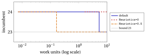
With the default parameters, a solution of \(24\) bins is found at once, and the optimal one only after \(2533\) nodes. Spending more effort in the heuristics (Heuristics=0.5 or MIPFocus=1) finds \(23\) at the root, about \(30\) times faster; without heuristics the first solution arrives after \(1.61\) work units, and the optimum is not found within the limit. Since the bound is \(23\) from the root, the whole difficulty of this instance is primal: finding the solution, not proving it optimal.
- The numbers depend on the instance, on the version of the solver and on the machine; a single instance proves nothing (chapter «Heuristic algorithms: definitions»). The lesson is qualitative: on instances whose bound is strong, as the BPP with \(LB=z(I)\), the time to solve is the time to find a good solution, and the heuristics of the solver — or a good MIP start — decide it.
33.9 What the MIP-based heuristics give
-
The chapter «Heuristic algorithms: definitions» ended with a warning: a heuristic gives only one side of the gap, and without a dual bound nothing can be said about the quality of its solution. The heuristics of the previous chapters give only primal bounds.
-
A MIP-based heuristic works with a MIP model, and the model comes with its LP relaxation; run inside a MIP solver, it comes with the dual bound of the branch-and-bound as well. For the first time, the heuristic knows how far it is from the optimum while it runs: the gap of the chapter «Heuristic algorithms: definitions» is computed at every moment, and when it is \(0\) the solution is proved optimal.
| heuristics of the previous chapters | MIP-based heuristics | |||||
|---|---|---|---|---|---|---|
| instance | solution | dual bound | gap | solution | dual bound | gap |
| KP | \(GR\): \(16\) | LP: \(17\) | \(6.25\%\) | LB, PS: \(17\) | PS: \(17\) | \(0\%\) |
| BPP | \(FF\): \(4\) | \(\lceil 21/7\rceil=3\) | \(33.3\%\) | pump (seed \(7\)): \(3\) | LP: \(3\) | \(0\%\) |
| TSP | \(NN\): \(25\) | two-edge: \(17\) | \(47.1\%\) | rounding: \(18\) | LP: \(18\) | \(0\%\) |
| \(P\,||\,C_{\max}\) | \(LPT\): \(11\) | \(9\) | \(22.2\%\) | RINS, LB, PS: \(9\) | LP: \(9\) | \(0\%\) |
| lot sizing, capacitated | RF: \(170\) | LP: \(102.38\) | \(66.0\%\) | FO: \(160\) | solver: \(160\) | \(0\%\) |
| medium BPP | \(FFD\): \(24\) | \(23\) | \(4.3\%\) | Gurobi: \(23\) | \(23\) | \(0\%\) |
- On the KP the integer rounding of the LP value is \(\lfloor 17.75\rfloor=17\), and proximity search proves the optimality of \(17\) by itself, by the optimality condition of proximity search (Chapter 10 «MIP heuristics» of the module Integer Linear Programming). On the capacitated lot sizing instance the LP bound is weak, and the gap is closed by the branch-and-bound of the solver, which proves that \(160\) is optimal.
A MIP-based heuristic does not only find solutions: inside a MIP solver it works with a dual bound, so the gap of its solution is always known, and a gap equal to \(0\) certifies optimality.
33.10 Typical mistakes
Warning
-
Rounding a problem with equality constraints. Independent roundings of an assignment constraint almost never sum to \(1\): on the BPP and on \(P\,||\,C_{\max}\) rounding fails.
-
Believing that a dive can undo a decision. A dive is one path of the tree, without backtracking: the first wrong fixing (on the KP, \(x_2:=0\)) is never revised.
-
Using the feasibility pump to get a good solution. After the first LP the pump ignores the objective: it returns a feasible solution, possibly with empty bins left open.
-
Trusting hard fixing. RINS fixes the variables on which the LP and the incumbent agree, so it cannot find a better solution that changes one of them.
-
Forgetting the cutoff constraint. Without \(f(\vet x)\le f(\bar{\vet x})-\theta\) the sub-MIP returns the incumbent solution again; with it, an infeasible sub-MIP proves a local optimum.
-
Claiming optimality without the conditions. The optimality condition of proximity search (Chapter 10 «MIP heuristics» of the module Integer Linear Programming) needs \(\theta=1\) and integer objective values on all the feasible solutions.
-
Ignoring the myopia of relax-and-fix. The relaxed future is optimistic: a decision that looks cheap can force a setup later.
-
Generalizing from one instance or one solver run. Paths and times depend on the version of the solver and on the tie-breaking rules, so the lessons are qualitative.
33.11 In summary
In summary
-
The MIP-based heuristics of Chapter 10 «MIP heuristics» of the module Integer Linear Programming apply to the classical problems through their MIP models.
-
Rounding and diving build a solution from the LP; the feasibility pump looks only for feasibility; RINS, local branching and proximity search improve an incumbent solution with a sub-MIP.
-
Relax-and-fix builds a solution along the time, fix-and-optimize improves it window by window.
-
Inside a MIP solver the dual bound is available: the gap of the heuristic solution is known, and a gap equal to \(0\) certifies optimality.
Dashboard of the reference instances. Best solution found by the methods of this chapter against the dual bound (\(\max\) for the KP, \(\min\) for the others):
| instance | solution | dual bound | gap |
|---|---|---|---|
| KP | \(17\) | \(17\) | \(0\%\) |
| BPP | \(3\) | \(3\) | \(0\%\) |
| \(P\,||\,C_{\max}\) | \(9\) | \(9\) | \(0\%\) |
| lot sizing, capacitated | \(160\) | \(160\) | \(0\%\) |
| medium BPP | \(23\) | \(23\) | \(0\%\) |
The code of the chapter, in Python with gurobipy (the models of the four problems, the heuristics and the experiment with the parameters of Gurobi), runs every example of the chapter and every instance of the exercises in the Colab notebook of the chapter.
Exercises on this chapter: MIP heuristics