4. Constructive heuristics
Class: algorithms · Script: python/cap05_heuristics.py, python/euristiche.py

A constructive heuristic builds one solution quickly, adding one element at a time and never backtracking. It proves nothing about the quality of that solution, and it is not even guaranteed to reach a feasible one: it can get stuck part-way, with an element that fits nowhere. When it does end with a feasible solution, that solution is the other half of the sandwich of chapter 2: the pessimistic side, the one guaranteed by a solution that really exists; when it fails, there is no primal bound.
What a heuristic must produce in this course
- a readable pseudocode, with the scanning order, the choice criterion, the tie-breaking rule and the failure case stated;
- the corresponding Python function, line by line;
- the trace of the execution on an instance;
- the feasibility check: constraints, bounds and integrality;
- the resulting bound, with the right name.
Point 4 is not a formality: a solution satisfying the linear constraints but with a fractional component is feasible for the relaxation, not for the MILP, and its value is not a primal bound.
The side of the bound depends on the objective, not on the heuristic
In a minimisation the value of a feasible solution is an upper bound: \(z(\mathit{MILP}) \le \mathit{UB}\). In a maximisation it is a lower bound: \(\mathit{LB} \le z(\mathit{MILP})\). Calling \(UB\) the result of a constructive heuristic on a maximisation is the commonest sign error in the course.
Bin packing: the insertion rules
The classical problem is bin packing, whose model is in the solver chapter: items must be put into identical bins of limited capacity, using as few of them as possible. Here it is not solved: it is built, one choice at a time.
Build(n, k, t, a, gamma):
  x[j][m] <- 0 for every j, m;   ra[m] <- a[m] for every m
  for j = 1..n:
      # next-fit:  the current machine only, then the next one
      # first-fit: the first m with t[j][m] <= ra[m]
      # best-fit:  among the feasible m, the one with smallest gamma(j,m,ra)
      choose m* by the rule
      if no m is feasible: return "no solution found"
      x[j][m*] <- 1;  ra[m*] <- ra[m*] - t[j][m*]
  return x
All three scan the jobs in the given order: changing the order changes the result, and this must be said when a value is reported. Ties are broken on the smallest index, so the run is reproducible.
On a small assignment instance (a minimisation):
| Heuristic | \(UB\) | \(z(\mathit{MILP})\) | heuristic gap |
|---|---|---|---|
| next-fit | 14 | 11 | \(27.3\%\) |
| first-fit | 14 | 11 | \(27.3\%\) |
| best-fit on cost | 11 | 11 | \(0.0\%\) |
The best-fit on cost finds the optimum; but no bound certifies it — that takes the solver, or a dual bound reaching \(11\), and there the hand-built dual stops at \(10\).
\(P||C_{\max}\): the least loaded rule
The second classic is scheduling on identical machines, written \(P||C_{\max}\): \(n\) jobs of duration \(t_j\) over \(k\) identical machines, minimising the instant the last one finishes. The natural rule is list scheduling — the current job goes to the least loaded machine — and the order in which the jobs are looked at decides the result. The best order is by decreasing duration, and the rule it gives is called LPT.
LPT(n, k, t):
  L[m] <- 0 for every m                       # current loads
  for j in order of DECREASING t[j]:
      m* <- argmin_m L[m]                     # ties: the smallest index
      x[j][m*] <- 1;  L[m*] <- L[m*] + t[j]
  return x, max_m L[m]
The decreasing order is essential: leaving the long jobs for last makes them impossible to place.
Seven jobs on three machines
\(t = (5, 5, 4, 4, 3, 3, 3)\), \(k = 3\), total \(27\).
- Steps 1–3. The jobs \(5\), \(5\), \(4\) go to the three empty machines: \(L = (5, 5, 4)\).
- Step 4. Job \(4\): the smallest load is machine 3, which goes to \(8\). \(L = (5, 5, 8)\).
- Steps 5–6. The two jobs of length \(3\) go to machines 1 and 2: \(L = (8, 8, 8)\).
- Step 7. The last job of length \(3\) finds all loads equal to \(8\); by the tie rule it goes to machine 1, which reaches \(11\).
LPT makespan: \(\mathit{UB} = 11\), with loads \((11, 8, 8)\).
The elementary bound. The makespan is at least \(\max(\max_j t_j,\ \sum_j t_j / k) = \max(5, 9) = 9\). The optimum is exactly \(z(\mathit{MILP}) = 9\) — attained with \(\{5,4\}\), \(\{5,4\}\), \(\{3,3,3\}\) — and LPT is off by \(22.2\%\).
Two free bounds, to be compared
\(\max_j t_j\) and \(\sum_j t_j / k\) are computable without solving anything, and the better of the two is often already close to the optimum. An "obvious" bound nobody writes down is a wasted bound: the dual of chapter 2 is for when the obvious ones are not enough, not instead of them.
Set covering: the cheapest completion rule
CoveringHeuristic(c, S):
  uncovered <- {1..m};   y[j] <- 0 for every j
  while uncovered is not empty:
      for every j not yet chosen: new(j) <- |{i in uncovered : j in S_i}|
      if new(j) = 0 for every j: return "no solution found"
      j* <- argmin_{j : new(j) > 0} c[j] / new(j)
      y[j*] <- 1;   uncovered <- uncovered \ {i : j* in S_i}
  return y
The criterion is the cost per newly covered zone, not the absolute cost.
On the four teams of chapter 2, \(c = (4,3,5,3)\): step 1 ratios \(4/3\), \(1\), \(5/3\), \(1\) → element 2 (covers zones 1, 2, 5); step 2 ratios \(2\), \(5/2\), \(3/2\) → element 4 (zones 4 and 6); step 3 ratios \(4\) and \(5\) → element 1. Solution \(\{1,2,4\}\), cost \(\mathit{UB} = 10\), which here is the optimum.
Knapsack: the best ratio rule
The knapsack is the model the solver chapter opens with: the items have a value as well as a weight, and there is a single resource. The constructive rule looks at the ratio between the two, and what it produces is a feasible solution, hence a primal bound.
KnapsackHeuristic(p, w, C):
  residual <- C;   y[j] <- 0 for every j
  for j in order of DECREASING p[j]/w[j]:
      if w[j] <= residual:  y[j] <- 1;  residual <- residual - w[j]
  return y
On \(p = (10,7,6,4)\), \(w = (5,4,3,3)\), \(C = 9\): ratios \(2\), \(7/4\), \(2\), \(4/3\); items 1 and 3 are taken (weight \(8\)), value \(16\). Since the problem is a maximisation, \(\mathit{LB} = 16 \le z(\mathit{MILP}) = 17\), gap \(5.9\%\): the optimum takes items 1 and 2, filling the knapsack exactly. The constructive heuristic goes wrong because item 3 leaves an unusable residual.
TSP: the nearest neighbour
The fourth classic is the travelling salesman problem (TSP): given \(n\) cities and the distances \(d_{ij}\) between every pair, find the shortest tour that visits them all once and returns to the start. It is the problem where step-by-step construction shows best, because the solution is a sequence: the order is the solution.
The classical constructive rule is the nearest neighbour: start from a city and each time go to the nearest among those not yet visited; when none are left, return to the start. It is feasible by construction and fast, because at each step it looks only at the distances from the current city.
Five cities, five starting points
The distances, symmetric:
| 1 | 2 | 3 | 4 | 5 | |
|---|---|---|---|---|---|
| 1 | — | 5 | 2 | 2 | 9 |
| 2 | 5 | — | 4 | 3 | 4 |
| 3 | 2 | 4 | — | 4 | 7 |
| 4 | 2 | 3 | 4 | — | 7 |
| 5 | 9 | 4 | 7 | 7 | — |
Starting from city 1: the nearest is 3 (distance 2); from there 2 (4); then 4 (3); 5 is left (7); and the return to 1 costs 9. The tour \(1 \to 3 \to 2 \to 4 \to 5 \to 1\) has length 25.
The last arc is the one that is paid for: the rule chooses well while it has a choice, and at the last step it has none. Changing the starting city changes the tour:
| start | tour | length |
|---|---|---|
| 1 | \(1 \to 3 \to 2 \to 4 \to 5 \to 1\) | 25 |
| 2 | \(2 \to 4 \to 1 \to 3 \to 5 \to 2\) | 18 |
| 3 | \(3 \to 1 \to 4 \to 2 \to 5 \to 3\) | 18 |
| 4 | \(4 \to 1 \to 3 \to 2 \to 5 \to 4\) | 19 |
| 5 | \(5 \to 2 \to 4 \to 1 \to 3 \to 5\) | 18 |
With five cities the distinct tours are \((5-1)!/2 = 12\) and they can all be enumerated: the optimum is \(1 \to 3 \to 5 \to 2 \to 4 \to 1\), of length 18. Three starting points out of five find it, one stops at 19 and the one we started from at 25, that is 38.9 % above the optimum.
Two things to take away. The heuristic gives one feasible solution, hence an upper bound — here \(z(\mathit{MILP}) \le 25\) — and nothing else; that 18 is the optimum is known by enumeration. And running the same rule from every start, keeping the best tour, costs \(n\) times as much and gives a better bound: it is the simplest form of multi-start, and it is still a bound from one side only.
Lot sizing: least unit cost period covering
LeastUnitCost(d, f, h):
  t <- 1
  while t <= T:
      skip the periods with d[t] = 0
      for k = 1..T-t+1:
          Q_k <- sum of d[t..t+k-1]
          c_k <- (f + h * sum of (s-t)*d[s] for s = t..t+k-1) / Q_k
      k* <- argmin_k c_k                      # the lowest average cost per unit
      produce Q_{k*} in period t;   t <- t + k*
This is not the Wagner–Whitin procedure
Wagner–Whitin is an exact dynamic-programming algorithm for the uncapacitated lot-sizing model: it solves that model to optimality in polynomial time. The procedure above is a heuristic, and its value is only a bound. Calling it "the Wagner–Whitin constructive heuristic" confuses two different things.
On \(d = (20, 10, 30, 40, 10)\), setup \(f = 50\), holding \(h = 1\): from period 1 it pays to cover 2 periods (unit cost \(2\)); from period 3 another 2 (unit cost \(\approx 1.286\)); from period 5 only that one (unit cost \(5\)). Cost \(\mathit{UB} = 200\) against \(z(\mathit{MILP}) = 170\), gap \(17.6\%\) — which is also the value Wagner–Whitin would give, being exact on this model.
Local search, and what it does not give
A local search starts from a feasible solution and tries elementary moves, accepting those that improve; it stops at a local optimum.
On the LPT solution (\(L = (11, 8, 8)\), makespan \(11\)), the move "move one job to another machine" improves nothing: moving one of the two jobs of length \(3\) off machine 1 brings its load to \(8\) but raises the receiving machine to \(11\). The local search stops at \(11\), while the optimum is \(9\): to get there a swap between two machines is needed.
A local optimum is not a better bound
Local search returns a feasible solution, hence a bound on the pessimistic side, and nothing else. The fact that it stopped does not mean it has arrived.
When the constructive heuristic fails
«No solution found» is not «no solution exists»
Three jobs of duration \((3, 3, 2)\) on two machines with availability \((5, 3)\). Next-fit: job 1 goes to machine 1 (residual \(2\)); job 2 does not fit and moves to machine 2 (residual \(0\)); job 3 does not fit and there are no more machines: failure. But the problem is feasible: jobs 2 and 3 fit together on machine 1 (\(3 + 2 = 5\)) and job 1 on machine 2 (\(3 \le 3\)).
A constructive heuristic is myopic: it decides one thing at a time and
never backtracks. Its failure is information about the heuristic, not about
the problem. To prove a model infeasible one needs the solver
(Status = INFEASIBLE) or a proof.
The overview of the heuristics
| Heuristic | Direction | value | \(z(\mathit{MILP})\) | heuristic gap |
|---|---|---|---|---|
| next-fit / first-fit (assignment) | min (\(UB\)) | 14 | 11 | \(27.3\%\) |
| best-fit on cost (assignment) | min (\(UB\)) | 11 | 11 | \(0.0\%\) |
| LPT (makespan) | min (\(UB\)) | 11 | 9 | \(22.2\%\) |
| covering constructive heuristic | min (\(UB\)) | 10 | 10 | \(0.0\%\) |
| ratio constructive heuristic (knapsack) | max (\(LB\)) | 16 | 17 | \(5.9\%\) |
| least unit cost (lot sizing) | min (\(UB\)) | 200 | 170 | \(17.6\%\) |
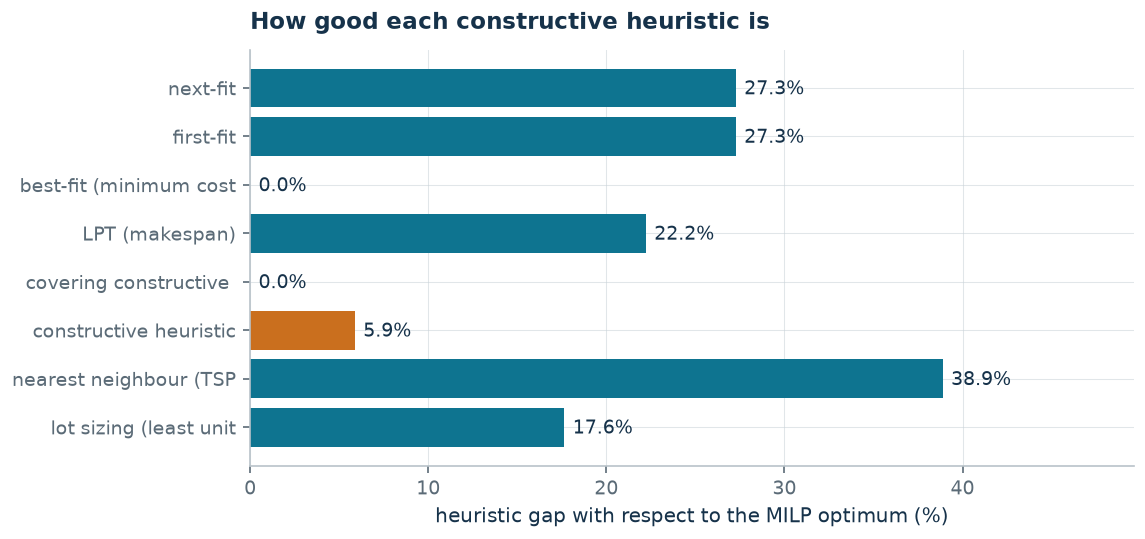
What this table teaches
Two heuristics find the optimum and four do not, and before solving the MILP there is no way of knowing which. A \(0\%\) gap and a \(27\%\) gap are told apart only afterwards. This is why the course always asks for two bounds: a heuristic on its own says how much a solution one can actually implement costs, not how much is being lost.
Code
The heuristics live in
python/euristiche.py,
the examples in
python/cap05_heuristics.py;
the notebook is
notebooks/cap05_heuristics.ipynb.
Show the complete script — python/cap05_heuristics.py (240 lines)
"""Chapter 4 -- Constructive heuristics on the classical problems, with trace and bound.

Every heuristic of the course on a minimal instance: the step-by-step trace (the
same text that ends up in the notes), the feasibility check of the solution
produced --- constraints, bounds *and* integrality --- and the comparison with
the optimum of the corresponding MILP. It ends with a local-search step and with
the case where the constructive heuristic fails although the problem is feasible.
"""
import gurobipy as gp
import pandas as pd
from gurobipy import GRB

from euristiche import (vicino_piu_vicino, best_fit, first_fit, euristica_copertura, euristica_lotti, euristica_zaino,
                        lpt, matrice, next_fit)
from mip import (ammissibile, frazione, nuovo_modello, rilassamento, risolvi,
                 stampa_soluzione, valuta, viola_interezza)
from stile import (ARANCIO, BLU, CICLO, GRIGIO, ROSSO, TEAL, VERDE, intestazione,
                   plt, salva_dati, salva_figura)

R = range
CONFRONTO = []


def confronta(nome, senso, valore_eur, zmilp, note=""):
    gap = abs(valore_eur - zmilp) / abs(zmilp) if abs(zmilp) > 1e-9 else 0.0
    ruolo = "ub" if senso == "min" else "lb"
    print(f"  {nome:34s} heuristic = {frazione(valore_eur):>6} ({ruolo})   "
          f"z(MILP) = {frazione(zmilp):>6}   gap = {100 * gap:.1f}%  {note}")
    CONFRONTO.append({"heuristic": nome, "sense": senso, "heuristic_value": valore_eur,
                      "role": ruolo, "z_milp": zmilp, "gap": gap})


# ---------- 1. BIN PACKING: NEXT-FIT, FIRST-FIT, BEST-FIT ----------
intestazione("5.1  The three bin-packing heuristics on jobs and machines")
t51 = [[2, 1, 3], [3, 4, 2], [4, 5, 3]]
c51 = [[5, 10, 2], [5, 4, 6], [5, 4, 6]]
a51 = [5, 6, 7]


def modello_assegnamento(t, c, a):
    n, k = len(t), len(a)
    m = nuovo_modello("assignment")
    x = m.addVars(n, k, vtype=GRB.BINARY, name="x")
    m.setObjective(gp.quicksum(c[j][mm] * x[j, mm] for j in R(n) for mm in R(k)), GRB.MINIMIZE)
    m.addConstrs((x.sum(j, "*") == 1 for j in R(n)), name="assign")
    m.addConstrs((gp.quicksum(t[j][mm] * x[j, mm] for j in R(n)) <= a[mm] for mm in R(k)),
                 name="availability")
    return m, x


m51, x51 = modello_assegnamento(t51, c51, a51)
z51 = risolvi(m51)
for nome, e in [("next-fit", next_fit(t51, a51)),
                ("first-fit", first_fit(t51, a51)),
                ("best-fit (minimum cost)", best_fit(t51, a51, lambda j, mm, ra: c51[j][mm], "cost"))]:
    valore = sum(c51[j][mm] for (j, mm) in e.x)
    sol = {f"x[{j},{mm}]": 1 for (j, mm) in e.x}
    assert ammissibile(m51, sol), nome           # constraints, bounds AND integrality
    confronta(f"5.1 {nome}", "min", valore, z51)
print("  Trace of the best-fit (the text that appears in the notes):")
best_fit(t51, a51, lambda j, mm, ra: c51[j][mm], "cost").traccia.stampa()

# ---------- 2. LPT: BALANCING OVER IDENTICAL MACHINES ----------
intestazione("5.2  LPT: the makespan on identical machines")
t52 = [5, 5, 4, 4, 3, 3, 3]
k52 = 3
e52 = lpt(t52, k52)
e52.traccia.stampa()
m52 = nuovo_modello("makespan")
x52 = m52.addVars(len(t52), k52, vtype=GRB.BINARY, name="x")
T52 = m52.addVar(name="T")
m52.setObjective(T52, GRB.MINIMIZE)
m52.addConstrs((x52.sum(j, "*") == 1 for j in R(len(t52))), name="assign")
m52.addConstrs((T52 >= gp.quicksum(t52[j] * x52[j, mm] for j in R(len(t52))) for mm in R(k52)),
               name="max")
z52 = risolvi(m52)
sol52 = {f"x[{j},{mm}]": 1 for (j, mm) in e52.x} | {"T": e52.makespan}
assert ammissibile(m52, sol52)
confronta("5.2 LPT (makespan)", "min", e52.makespan, z52,
          f"loads {[int(c) for c in e52.carichi]}, total {sum(t52)}")
print(f"  Elementary bound: the makespan is at least max(max_j t_j, total/k) = "
      f"max({max(t52)}, {frazione(sum(t52) / k52)}) = {frazione(max(max(t52), sum(t52) / k52))}")

# ---------- 3. COVERING GREEDY ----------
intestazione("5.3  Constructive covering heuristic")
c53 = [4, 3, 5, 3]
S53 = [[0, 1], [1, 2], [0, 2], [0, 3], [1, 3], [2, 3]]
e53 = euristica_copertura(c53, S53)
e53.traccia.stampa()
m53 = nuovo_modello("covering")
x53 = m53.addVars(len(c53), vtype=GRB.BINARY, name="x")
m53.setObjective(gp.quicksum(c53[j] * x53[j] for j in R(len(c53))), GRB.MINIMIZE)
m53.addConstrs((gp.quicksum(x53[j] for j in S53[i]) >= 1 for i in R(len(S53))), name="cover")
z53 = risolvi(m53)
assert ammissibile(m53, {f"x[{j}]": e53.y[j] for j in R(len(c53))})
confronta("5.3 covering constructive heuristic", "min", e53.valore, z53,
          f"chosen {[j + 1 for j in R(len(c53)) if e53.y[j]]}")

# ---------- 4. KNAPSACK GREEDY: A LOWER BOUND ----------
intestazione("5.4  Knapsack constructive heuristic: in a maximisation the heuristic gives a lower bound")
p54, w54, C54 = [10, 7, 6, 4], [5, 4, 3, 3], 9
e54 = euristica_zaino(p54, w54, C54)
e54.traccia.stampa()
m54 = nuovo_modello("knapsack")
x54 = m54.addVars(4, vtype=GRB.BINARY, name="x")
m54.setObjective(gp.quicksum(p54[j] * x54[j] for j in R(4)), GRB.MAXIMIZE)
m54.addConstr(gp.quicksum(w54[j] * x54[j] for j in R(4)) <= C54, name="capacity")
z54 = risolvi(m54)
assert ammissibile(m54, {f"x[{j}]": e54.y[j] for j in R(4)})
confronta("5.4 constructive heuristic by ratio p/w", "max", e54.valore, z54,
          f"taken {[j + 1 for j in R(4) if e54.y[j]]}, residual {e54.residuo:g}")

# ---------- 5. NEAREST NEIGHBOUR FOR THE TSP ----------
intestazione("5.5  Nearest neighbour for the TSP: the tour depends on the starting node")
# five cities, symmetric distances satisfying the triangle inequality
D55 = [[0, 5, 2, 2, 9],
       [5, 0, 4, 3, 4],
       [2, 4, 0, 4, 7],
       [2, 3, 4, 0, 7],
       [9, 4, 7, 7, 0]]
n55 = len(D55)
e55t = vicino_piu_vicino(D55, partenza=0)
e55t.traccia.stampa()
print(f"  Tour from node 1: {' -> '.join(str(v + 1) for v in e55t.tour)}, length {e55t.valore:g}")
tour_da = {}
for s in R(n55):
    e = vicino_piu_vicino(D55, partenza=s)
    tour_da[s] = (e.tour, e.valore)
    if s:
        print(f"  Tour from node {s + 1}: {' -> '.join(str(v + 1) for v in e.tour)}, "
              f"length {e.valore:g}")
from itertools import permutations
ottimo, tour_ottimo = None, None
for perm in permutations(R(1, n55)):
    if perm[0] > perm[-1]:
        continue
    giro = (0,) + perm + (0,)
    lung = sum(D55[giro[i]][giro[i + 1]] for i in R(n55))
    if ottimo is None or lung < ottimo:
        ottimo, tour_ottimo = lung, giro
print(f"  Optimum by enumeration: {' -> '.join(str(v + 1) for v in tour_ottimo)}, "
      f"length {ottimo:g}")
salva_dati(pd.DataFrame({"start": [s + 1 for s in R(n55)],
                         "tour": [" - ".join(str(v + 1) for v in tour_da[s][0]) for s in R(n55)],
                         "length": [tour_da[s][1] for s in R(n55)]}),
           "cap05_tsp")
confronta("5.5 nearest neighbour (TSP)", "min", e55t.valore, ottimo,
          f"tour {' - '.join(str(v + 1) for v in e55t.tour)}")

# ---------- 5. LOT SIZING GREEDY ----------
intestazione("5.6  Lot sizing: least unit cost period covering")
d55 = [20, 10, 30, 40, 10]
setup55, hold55 = 50, 1
e55 = euristica_lotti(d55, setup55, hold55)
e55.traccia.stampa()
T55 = len(d55)
m55 = nuovo_modello("lot_sizing")
q55 = m55.addVars(T55, name="q")
I55 = m55.addVars(T55, name="I")
y55 = m55.addVars(T55, vtype=GRB.BINARY, name="y")
Mtot = sum(d55)
m55.setObjective(gp.quicksum(setup55 * y55[t] + hold55 * I55[t] for t in R(T55)), GRB.MINIMIZE)
for t in R(T55):
    m55.addConstr((I55[t - 1] if t else 0) + q55[t] - I55[t] == d55[t], name=f"bilancio{t}")
    m55.addConstr(q55[t] <= Mtot * y55[t], name=f"link{t}")
z55 = risolvi(m55)
sol55 = {}
for t in R(T55):
    sol55[f"q[{t}]"] = e55.lanci.get(t, 0)
    sol55[f"y[{t}]"] = 1 if t in e55.lanci else 0
scorta = 0
for t in R(T55):
    scorta += sol55[f"q[{t}]"] - d55[t]
    sol55[f"I[{t}]"] = scorta
assert ammissibile(m55, sol55)
confronta("5.5 lot sizing (least unit cost)", "min", e55.valore, z55,
          f"runs in periods {[t + 1 for t in sorted(e55.lanci)]}")
print("  Wagner-Whitin solves this very model *to optimality* by dynamic programming:")
print(f"  its value is {frazione(z55)}, not the heuristic one.")

# ---------- 6. A LOCAL SEARCH STEP ----------
intestazione("5.7  A local-search step on the LPT solution")
carichi = list(e52.carichi)
assegn = {j: mm for (j, mm) in e52.x}
migliorato = True
passi = 0
while migliorato:
    migliorato = False
    for j, mm in list(assegn.items()):
        for nuovo in R(k52):
            if nuovo == mm:
                continue
            prova = list(carichi)
            prova[mm] -= t52[j]
            prova[nuovo] += t52[j]
            if max(prova) < max(carichi) - 1e-9:
                print(f"  Moving job {j + 1} from machine {mm + 1} to {nuovo + 1}: "
                      f"makespan {max(carichi):g} -> {max(prova):g}")
                carichi, assegn[j], migliorato, passi = prova, nuovo, True, passi + 1
                break
        if migliorato:
            break
if passi == 0:
    print(f"  No single move improves the makespan {max(carichi):g}: the LPT solution")
    print(f"  is a local optimum for this move. The global optimum is {frazione(z52)}.")
print("  A local optimum is not a global optimum, and local search produces no bound")
print("  better than that of the solution it returns.")

# ---------- 7. WHEN THE GREEDY FAILS ----------
intestazione("5.8  A failure of the constructive heuristic does not prove infeasibility")
t57 = matrice([3, 3, 2], 2)
a57 = [5, 3]
e57 = next_fit(t57, a57)
e57.traccia.stampa()
print(f"  next-fit: ok = {e57.ok}")
m57, x57 = modello_assegnamento(t57, [[1, 1], [1, 1], [1, 1]], a57)
z57 = risolvi(m57)
print(f"  The MILP, however, is feasible, with optimum {frazione(z57)}: solution "
      + ", ".join(f"x[{j+1}][{mm+1}]" for j in R(3) for mm in R(2) if x57[j, mm].X > 0.5))
print("  The constructive heuristic fails because it is myopic, not because the problem has no")
print("  solution: 'no solution found' is not 'no solution exists'.")
assert not e57.ok

# ---------- 8. THE OVERVIEW ----------
intestazione("5.9  The overview")
tab = pd.DataFrame(CONFRONTO)
salva_dati(tab, "cap05_euristiche")
fig, ax = plt.subplots(figsize=(7.6, 3.6))
etichette = [r["heuristic"].split(" ", 1)[1][:22] for r in CONFRONTO]
gap = [100 * r["gap"] for r in CONFRONTO]
colori = [TEAL if r["sense"] == "min" else ARANCIO for r in CONFRONTO]
ax.barh(etichette, gap, color=colori)
for i, g in enumerate(gap):
    ax.annotate(f"{g:.1f}%", (g, i), textcoords="offset points", xytext=(4, -3), fontsize=9)
ax.set_xlabel("heuristic gap with respect to the MILP optimum (%)")
ax.set_title("How good each constructive heuristic is")
ax.invert_yaxis()
ax.set_xlim(0, max(gap) * 1.25 + 1)
salva_figura(fig, "cap05_gap")
print("Done.")