2. Relaxations, duality and bounds
Class: LP · MILP · Script: python/cap04_bounds.py
This chapter teaches how to produce, by hand, a number that certainly lies on one side of the integer optimum. It serves three purposes: understanding how good a model is, how good a heuristic is, and how to read the numbers a solver reports when it has not finished.
What a relaxation is
A relaxation of \(\min\{c'x : x \in X\}\) is a problem \(\min\{c'x : x \in \hat X\}\) with \(X \subseteq \hat X\): the minimum over a larger set cannot be higher. In a maximisation the inequality is reversed.
| Name | What is dropped | Note |
|---|---|---|
| \(z(\mathit{LP})\), pure | \(x \in \{0,1\}\) becomes \(x \ge 0\) | this is the one whose dual is written by hand: fewer constraints, hence a dual with fewer variables |
| \(z(\mathit{LP}^+)\), bounds kept | \(x \in \{0,1\}\) becomes \(0 \le x \le 1\) | this is Gurobi's relax() and the root relaxation |
| \(z(\mathit{LP}^{++})\), strengthened | as above, plus valid inequalities | see below |
In a minimisation \(z(\mathit{LP}) \le z(\mathit{LP}^+) \le z(\mathit{LP}^{++}) \le z(\mathit{MILP})\).
The two relaxations coincide more often than one thinks
If the model contains an assignment constraint \(\sum_m x_{jm} = 1\) with \(x \ge 0\), then \(x_{jm} \le 1\) is already implied and the two relaxations are equal. In the bound table of chapter 7 this happens in problems 1, 4, 6 and 7.
The primal/dual conversion table
Minimisation primal, constraints indexed by \(i\), variables by \(j\):
| In the primal (min) | In the dual (max) |
|---|---|
| constraint \(i\) of type \(\ge\) | variable \(\pi_i \ge 0\) |
| constraint \(i\) of type \(\le\) | variable \(\pi_i \le 0\) |
| equality constraint \(i\) | free variable \(\pi_i\) |
| variable \(x_j \ge 0\) | constraint \(j\) of type \(\le c_j\) |
| free variable \(x_j\) | equality constraint \(j\), \(= c_j\) |
The dual objective is \(\max \sum_i b_i \pi_i\). If the primal is a maximisation, every direction is reversed and the dual is a minimisation.
Dual constraint \(j\) says: "the value I attach to the resources consumed by activity \(j\) cannot exceed its cost". With this reading, every recipe for building a dual solution has an economic meaning.
Weak duality, strong duality
- Weak duality: \(\sum_i b_i \bar\pi_i \le \sum_j c_j \bar x_j\) for every pair of feasible solutions. Always, with no assumptions. This is the one we need: it gives a lower bound from any feasible dual solution, even one built by hand.
- Strong duality: if the relaxation has a finite optimum, \(z(\mathit{D}(\mathit{LP})) = z(\mathit{LP})\). It
serves as a check: the optimum of the dual written by hand must coincide
with \(z(\mathit{LP})\). The course scripts verify it with an
assert.
And then: since every feasible solution of the MILP is feasible for the relaxation too,
There is no such thing as «the dual of the MILP»
The dual one writes is that of the relaxation. A MILP has no linear dual, and strong duality between a MILP and any linear program does not hold in general: the jump \(z(\mathit{MILP}) - z(\mathit{LP})\) is precisely what is missing.
Three recipes for building a dual solution by hand
- Zero out and saturate. Set all dual variables to zero except one family, and push those to the largest feasible value. In problem 7.1: \(\bar\pi = 0\) and \(\bar\mu_j = \min_m c_{jm}\), that is "every job costs at least its cheapest option".
- Constructive heuristic on the constraints. Scan the primal constraints one at a time, raise the corresponding dual variable until the first dual constraint that opposes it becomes tight, and update the residuals.
- The best ratio. With a single capacity constraint in a maximisation, \(\bar v = \max_j p_j / w_j\) is feasible and gives the bound \(b \bar v\).
Whichever recipe is used, the solution must be checked feasible for the dual — that is the only thing that makes the bound valid — and its value compared with \(z(\mathit{LP})\).
A minimisation problem, in full
Minimum-cost zone covering
A town has \(4\) districts; activating the team of district \(j\) costs \(c_j\). There are \(6\) sensitive zones, each on the border between two districts: zone \(i\) is covered if at least one of the two neighbouring teams is active. All zones must be covered at minimum cost.
Data \(c = (4, 3, 5, 3)\); the six zones are the six pairs of districts, in the order \(\{1,2\}\), \(\{2,3\}\), \(\{1,3\}\), \(\{1,4\}\), \(\{2,4\}\), \(\{3,4\}\).
The dual of the relaxation without the bounds, with \(\pi_i \ge 0\) for every covering constraint:
For the instance, every team covers three zones: \(\pi_1 + \pi_3 + \pi_4 \le 4\), \(\pi_1 + \pi_2 + \pi_5 \le 3\), \(\pi_2 + \pi_3 + \pi_6 \le 5\), \(\pi_4 + \pi_5 + \pi_6 \le 3\).
A dual solution by hand (recipe 2).
- Zone 1 (\(\{1,2\}\)): residuals \((4,3,5,3)\), the smallest among teams 1 and 2 is \(3\). \(\bar \pi_1 = 3\); residuals \((1,0,5,3)\).
- Zone 2 (\(\{2,3\}\)): the residual of team 2 is \(0\), so \(\bar \pi_2 = 0\).
- Zone 3 (\(\{1,3\}\)): the smallest of \(1\) and \(5\) is \(1\). \(\bar \pi_3 = 1\); residuals \((0,0,4,3)\).
- Zones 4 and 5: teams 1 and 2 have zero residual, so \(\bar \pi_4 = \bar \pi_5 = 0\).
- Zone 6 (\(\{3,4\}\)): the smallest of \(4\) and \(3\) is \(3\). \(\bar \pi_6 = 3\).
A primal upper bound. The covering constructive heuristic — at each step one picks the element costing least per newly covered requirement — takes teams \(1\), \(2\), \(4\), of cost \(4+3+3 = 10\): a feasible and integer solution, so \(\mathit{UB} = 10\).
| \(UB\) (constructive heuristic) | \(LB\) (dual by hand) | \(z(\mathit{LP})\) | \(z(\mathit{MILP})\) | heuristic gap |
|---|---|---|---|---|
| 10 | 7 | \(15/2\) | 10 | \(0.0\%\) |
The certified gap between the two hand-built bounds is \((10-7)/10 = 30\%\): without solving the MILP we would know only that the optimum lies between \(7\) and \(10\). The heuristic was already optimal, but the bounds cannot tell us that.
A maximisation problem: the roles swap
Knapsack with several resources
Five jobs of value \(p = (10, 9, 7, 6, 4)\) and three resources — steel, lathe hours and testing hours — of availability \(b = (10, 9, 8)\). The consumptions are \(a_{1\cdot} = (6, 4, 3, 3, 2)\), \(a_{2\cdot} = (1, 3, 4, 2, 3)\) and \(a_{3\cdot} = (3, 2, 2, 4, 1)\): one row per resource, one column per job.
With \(x_j = 1\) if job \(j\) is done, the primal maximises \(\sum_j p_j x_j\) under one capacity row per resource. The dual of the relaxation without the bounds therefore has one variable per resource, \(v_i \ge 0\): it minimises \(\sum_i b_i v_i\) with \(\sum_i a_{ij} v_i \ge p_j\) for every job. Each dual constraint now has three terms, one per resource, because the column of \(x_j\) in the primal has three rows.
- Heuristic (by ratio of value to total consumption): the ratios are \(1\), \(1\), \(7/9\), \(6/9\) and \(4/6\); jobs 1 and 2 are taken, and nothing else fits because the steel has run out. Value \(19\). In a maximisation the heuristic gives a lower bound: \(\mathit{LB} = 19\).
- Dual by hand (recipe 3, adapted): one pays a single resource. Setting \(\bar v_i = \max_j p_j / a_{ij}\) and all the others to zero, every dual constraint is satisfied by the single term \(a_{ij} \bar v_i \ge p_j\). The three choices give \(70/3\) with the steel, \(90\) with the lathe and \(36\) with the testing: the cheapest is the steel. In a maximisation the dual gives an upper bound: \(\mathit{UB} = 70/3 \approx 23.33\).
The optimum picks jobs 2, 3 and 4, which saturate all three resources. Here the dual by hand is not optimal for the relaxation (\(70/3 > 159/7\)): paying a single resource is a valid recipe, but a coarse one, because it ignores that the other two are saturated as well. The relaxation with the bounds kept is worth \(22\) and coincides with the integer optimum.
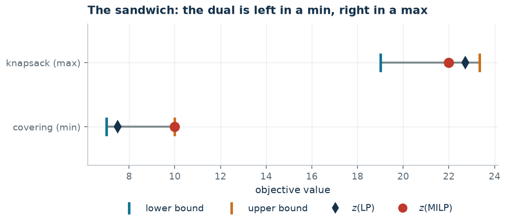
The sandwich, written once and for all
where \((\bar\pi_1, \bar\pi_2, \dots, \bar\pi_m)\) is a feasible dual solution of the relaxation, of value \(\sum_{i=1}^{m} b_i\, \bar\pi_i\), and \((\bar x_1, \bar x_2, \dots, \bar x_n)\) a feasible solution of the MILP, of value \(\sum_{j=1}^{n} c_j\, \bar x_j\).
The relaxation side is optimistic and holds all the dual bounds; the heuristic side is pessimistic and holds all the feasible solutions. The name (\(\mathit{LB}\) or \(\mathit{UB}\)) depends on the direction of the objective, the role does not.
Valid inequalities and constraints that preserve optimality
- A valid inequality is satisfied by all feasible integer solutions: adding it does not change \(z(\mathit{MILP})\); if it reduces \(z(\mathit{LP}^+)\) it is called a cut.
- A constraint that preserves optimality cuts off some feasible solutions but not all the optimal ones. It is not a valid inequality, and must be declared as such (example: \(z_j \le M_j y_j\) in an activation binary).
The cover cut. A set \(S\) is a cover if \(\sum_{j \in S} w_j > b\); then \(\sum_{j \in S} x_j \le |S| - 1\) is valid. On the knapsack (\(w = (5,4,3,3)\), \(b = 9\)) the minimal covers are the four triples. The optimal solution of the relaxation is \(\tilde x = (1,\ 1/4,\ 1,\ 0)\):
| Cover \(S\) | \(\sum_{j \in S} \tilde x_j\) | \(\|S\|-1\) | |
|---|---|---|---|
| \(\{1,2,3\}\) | \(9/4\) | 2 | violated: the cut is needed |
| \(\{1,2,4\}\) | \(5/4\) | 2 | satisfied |
| \(\{1,3,4\}\) | \(2\) | 2 | satisfied (with equality) |
| \(\{2,3,4\}\) | \(5/4\) | 2 | satisfied |
Adding the four cuts, \(z(\mathit{LP}^+)\) drops from \(71/4 = 17.75\) to \(69/4 = 17.25\) and \(z(\mathit{MILP})\) stays \(17\).
Stronger formulations
Two formulations \(A\) and \(B\) are compared in two steps: (1) same integer set, that is the two formulations must admit exactly the same points with integer coordinates — without this nothing is being compared; (2) \(B\) is stronger if \(X_B \subseteq X_A\) as polyhedra. The reference case is activation.
Stronger does not mean faster
A stronger formulation has fewer nodes but more rows, and every node costs more. What can be proved is the strength of the relaxation; speed is measured.
What the solver says
ObjBound is not the root relaxation
On the covering instance, the relaxation of the model as we wrote it is
\(15/2\) and the integer optimum \(10\). Yet Gurobi reports ObjBound = 10 and
NodeCount = 0: it closed the gap at the root, with presolve, its own cuts
and heuristics, without ever branching. Switching those off
(Presolve = Cuts = Heuristics = 0) the same model gives the same optimum
but with \(5\) nodes.
Two consequences: "how hard a model is" is not a property of the model
alone; and the relaxation we speak of in the hand-built bounds is that of
the model as written, obtained with relax().
LP duals are not the marginal prices of the MILP
| \(b\) | \(z(\mathit{MILP})\) | \(z(\mathit{LP}^+)\) | LP dual | true change |
|---|---|---|---|---|
| 8 | 16 | 16 | \(2\) | — |
| 9 | 17 | \(71/4\) | \(7/4\) | \(+1\) |
| 10 | 17 | \(39/2\) | \(7/4\) | 0 |
| 11 | 20 | \(85/4\) | \(7/4\) | \(+3\) |
| 12 | 23 | 23 | \(7/4\) | \(+3\) |
The LP dual is the ratio \(p_j/w_j\) of the "critical" item. The true change of the integer optimum comes in jumps: from \(b = 9\) to \(b = 10\) it does not change at all, while the dual promises \(7/4\).
What can be said, then
Of the LP dual, the only use this course makes of it remains true: it is a bound. As managerial advice ("is it worth buying one more unit?") it must be checked by solving the MILP again: the difference \(z(\mathit{MILP})(b_i + 1) - z(\mathit{MILP})(b_i)\) is the only correct answer, and there is no closed formula for it.
The bound protocol of the course
Every problem of the course produces: (1) a feasible and integer solution from a heuristic, checked on constraints, bounds and integrality; (2) the dual of the relaxation without the bounds, in general form and for the instance; (3) a feasible dual solution built by hand, with the recipe declared; (4) the two relaxations from the solver; (5) the optimum and the table \(\mathit{UB} \cdot \mathit{LB} \cdot z(\mathit{LP}) \cdot z(\mathit{LP}^+) \cdot z(\mathit{MILP}) \cdot\) gap; (6) the additional considerations.
Every number in the table exists in a CSV produced by the problem's script, and
an assert in check_numbers.py compares it with the value quoted in the text.
Code
The complete script is
python/cap04_bounds.py;
the notebook is
notebooks/cap04_bounds.ipynb.
Show the complete script — python/cap04_bounds.py (285 lines)
"""Chapter 2 -- Relaxations, duality and bounds: the checked examples.

A minimisation and a maximisation problem, written with their duals; a dual
solution built by hand and the check of weak duality; the comparison between the
relaxation without the bounds and the one with the bounds kept; a cover cut; the
bound read from Gurobi at the end of the solve; and the counterexample showing why the
LP duals are not the marginal prices of the MILP.
"""
import gurobipy as gp
import pandas as pd
from gurobipy import GRB

from mip import (ammissibile, due_rilassamenti, frazione, nuovo_modello, registra_bound,
                 rilassamento, risolvi, stampa_soluzione, valuta, viola_interezza)
from stile import (ARANCIO, BLU, CICLO, GRIGIO, ROSSO, TEAL, VERDE, intestazione,
                   plt, salva_dati, salva_figura)

R = range

# ---------- 1. A MINIMISATION, ITS DUAL, A DUAL SOLUTION BUILT BY HAND ----------
intestazione("4.1  Minimum-cost covering: primal, dual and a bound built by hand")
# min sum c_j x_j   s.t.  sum_{j in S_i} x_j >= 1 for every i,  x binary
c41 = [4, 3, 5, 3]                       # cost of the four teams
# six zones, each on the border between two districts: zone i is covered by the
# two teams of the districts it borders
S41 = [[0, 1], [1, 2], [0, 2], [0, 3], [1, 3], [2, 3]]
n41, m41 = len(c41), len(S41)


def primale_41():
    m = nuovo_modello("covering")
    x = m.addVars(n41, vtype=GRB.BINARY, name="x")
    m.setObjective(gp.quicksum(c41[j] * x[j] for j in R(n41)), GRB.MINIMIZE)
    m.addConstrs((gp.quicksum(x[j] for j in S41[i]) >= 1 for i in R(m41)), name="cover")
    return m, x


def duale_41():
    """max sum u_i  s.t.  sum_{i : j in S_i} u_i <= c_j,  u >= 0."""
    d = nuovo_modello("dual_covering")
    u = d.addVars(m41, name="u")
    d.setObjective(u.sum(), GRB.MAXIMIZE)
    d.addConstrs((gp.quicksum(u[i] for i in R(m41) if j in S41[i]) <= c41[j] for j in R(n41)),
                 name="rc")
    return d, u


m41p, x41 = primale_41()
z41 = risolvi(m41p)
scelte41 = [j + 1 for j in R(n41) if x41[j].X > 0.5]
print(f"  Integer optimum: z(MILP) = {frazione(z41)}, teams chosen {scelte41}")

# dual solution built by hand: each zone gets the smallest unit cost still
# available, respecting the dual constraints one column at a time (dual constructive heuristic)
u_mano = {i: 0.0 for i in R(m41)}
residuo = {j: c41[j] for j in R(n41)}
for i in R(m41):
    incremento = min(residuo[j] for j in S41[i])
    u_mano[i] = incremento
    for j in S41[i]:
        residuo[j] -= incremento
d41, u41 = duale_41()
lb41, viol = valuta(d41, {f"u[{i}]": u_mano[i] for i in R(m41)})
assert viol <= 1e-9, viol
print("  Dual solution by hand (constructive heuristic on the zones): u = "
      + ", ".join(f"u_{i+1} = {frazione(u_mano[i])}" for i in R(m41))
      + f"   ->  lb = {frazione(lb41)}")
zlp41, zlp41r, pi41 = due_rilassamenti(m41p, d41)
print(f"  Weak duality checked: {frazione(lb41)} <= {frazione(zlp41)} <= "
      f"{frazione(z41)}")
assert lb41 <= zlp41 + 1e-9 <= z41 + 1e-9
# primal upper bound: the covering constructive heuristic (one uncovered zone at a time)
scoperte = set(R(m41))
presi41 = []
while scoperte:
    j = min(R(n41), key=lambda j: c41[j] / max(1, len({i for i in scoperte if j in S41[i]}))
            if any(j in S41[i] for i in scoperte) else float("inf"))
    presi41.append(j)
    scoperte -= {i for i in scoperte if j in S41[i]}
ub41_primale = sum(c41[j] for j in presi41)
assert ammissibile(m41p, {f"x[{j}]": 1 for j in presi41})
print(f"  Constructive covering heuristic: teams {sorted(j + 1 for j in presi41)}, "
      f"ub = {frazione(ub41_primale)}")
riga41 = registra_bound("minimum-cost covering", ub41_primale, lb41, zlp41, zlp41r, z41)
salva_dati(pd.DataFrame([riga41]), "cap04_copertura")

# ---------- 2. A MAXIMISATION: THE ROLES SWAP ----------
intestazione("4.2  A knapsack with several resources: the heuristic gives the lower bound")
# Multidimensional knapsack: one capacity row per resource, not a single one. With
# one resource only the dual would have a single variable and one term per
# constraint, and the choice the recipe has to make would not show.
p42 = [10, 9, 7, 6, 4]                   # values
A42 = [[6, 4, 3, 3, 2],                  # steel used
       [1, 3, 4, 2, 3],                  # lathe hours
       [3, 2, 2, 4, 1]]                  # testing hours
B42 = [10, 9, 8]                         # availability of the three resources
NOMI42 = ["steel", "lathe", "testing"]
no42, nr42 = len(p42), len(B42)


def primale_42():
    m = nuovo_modello("knapsack")
    x = m.addVars(no42, vtype=GRB.BINARY, name="x")
    m.setObjective(gp.quicksum(p42[j] * x[j] for j in R(no42)), GRB.MAXIMIZE)
    m.addConstrs((gp.quicksum(A42[i][j] * x[j] for j in R(no42)) <= B42[i]
                  for i in R(nr42)), name="capacity")
    return m, x


def duale_42():
    """Dual of the relaxation without the bounds (x >= 0):
       min sum_i b_i v_i  s.t.  sum_i a_ij v_i >= p_j for every item,  v >= 0."""
    d = nuovo_modello("dual_knapsack")
    v = d.addVars(nr42, name="v")
    d.setObjective(gp.quicksum(B42[i] * v[i] for i in R(nr42)), GRB.MINIMIZE)
    d.addConstrs((gp.quicksum(A42[i][j] * v[i] for i in R(nr42)) >= p42[j]
                  for j in R(no42)), name="rc")
    return d, v


m42, x42 = primale_42()
z42 = risolvi(m42)
scelte42 = [j + 1 for j in R(no42) if x42[j].X > 0.5]
consumo = [sum(A42[i][j] for j in R(no42) if x42[j].X > 0.5) for i in R(nr42)]
print(f"  Integer optimum: z(MILP) = {frazione(z42)}, items {scelte42}")
print("  Consumption at the optimum: "
      + ", ".join(f"{NOMI42[i]} {consumo[i]} out of {B42[i]}" for i in R(nr42))
      + " --- all three resources are saturated.")
# constructive heuristic by value / total consumption: it gives a LOWER bound
ordine = sorted(R(no42), key=lambda j: -p42[j] / sum(A42[i][j] for i in R(nr42)))
presi, carico = [], [0] * nr42
for j in ordine:
    if all(carico[i] + A42[i][j] <= B42[i] for i in R(nr42)):
        presi.append(j)
        carico = [carico[i] + A42[i][j] for i in R(nr42)]
lb42 = sum(p42[j] for j in presi)
assert ammissibile(m42, {f"x[{j}]": 1 for j in presi})
print("  Constructive heuristic by value / total consumption: "
      f"it takes {sorted(j + 1 for j in presi)}, lb = {frazione(lb42)}")
# dual by hand: one pays a single resource, the one giving the lowest bound
d42, v42 = duale_42()
candidati = {}
for i in R(nr42):
    vi = max(p42[j] / A42[i][j] for j in R(no42))
    candidati[i] = B42[i] * vi
i_scelta = min(candidati, key=candidati.get)
v_scelta = max(p42[j] / A42[i_scelta][j] for j in R(no42))
mano = {f"v[{i}]": (v_scelta if i == i_scelta else 0.0) for i in R(nr42)}
ub42, viol = valuta(d42, mano)
assert viol <= 1e-9, viol
print("  Dual solution by hand: one pays a single resource. "
      + ", ".join(f"{NOMI42[i]} would give {frazione(candidati[i])}" for i in R(nr42)))
print(f"  The cheapest is {NOMI42[i_scelta]}, with v = {frazione(v_scelta)}  ->  "
      f"ub = {frazione(ub42)}")
zlp42, zlp42r, _ = due_rilassamenti(m42, d42)
print(f"  The sandwich of a maximisation: {frazione(lb42)} <= z(MILP) = {frazione(z42)} <= "
      f"z(LP) = {frazione(zlp42)} <= ub = {frazione(ub42)}")
assert lb42 <= z42 <= zlp42 + 1e-9 <= ub42 + 1e-9
riga42 = registra_bound("knapsack", ub42, lb42, zlp42, zlp42r, z42, senso="max")
salva_dati(pd.DataFrame([riga42]), "cap04_zaino")

# ---------- 3. A COVER CUT ----------
# Cover cuts are read one constraint at a time: here we go back to a knapsack with
# a single resource, smaller than the one of section 4.2.
p43 = [10, 7, 6, 4]                      # values
w43 = [5, 4, 3, 3]                       # weights
C43 = 9


def primale_43(C=C43):
    m = nuovo_modello("knapsack_one_resource")
    x = m.addVars(4, vtype=GRB.BINARY, name="x")
    m.setObjective(gp.quicksum(p43[j] * x[j] for j in R(4)), GRB.MAXIMIZE)
    m.addConstr(gp.quicksum(w43[j] * x[j] for j in R(4)) <= C, name="capacity")
    return m, x

intestazione("4.3  A valid inequality: the cover cut")
from itertools import combinations
tutte = [s for k in R(2, 5) for s in combinations(R(4), k) if sum(w43[j] for j in s) > C43]
coperture = [s for s in tutte                                   # only the minimal ones
             if all(sum(w43[j] for j in t) <= C43
                    for t in combinations(s, len(s) - 1))]
print("  Minimal covers found: "
      + "; ".join("{" + ", ".join(str(j + 1) for j in s) + "}" for s in coperture))
m43, x43 = primale_43()
z43_prima = risolvi(m43)   # the integer optimum before the cuts
zlp43_prima, sol43, _ = rilassamento(m43, rafforzato=True)
print("  Optimal solution of the relaxation without cuts: "
      + ", ".join(f"x_{j+1} = {frazione(sol43[f'x[{j}]'])}" for j in R(4)))
for s in coperture:
    somma = sum(sol43[f"x[{j}]"] for j in s)
    stato = "VIOLATED" if somma > len(s) - 1 + 1e-9 else "satisfied"
    print(f"    cut on {{{', '.join(str(j + 1) for j in s)}}}: "
          f"sum = {frazione(somma)} against {len(s) - 1}  ->  {stato}")
for s in coperture:
    m43.addConstr(gp.quicksum(x43[j] for j in s) <= len(s) - 1, name="cover" + "".join(map(str, s)))
z43 = risolvi(m43)
zlp43_dopo, _, _ = rilassamento(m43, rafforzato=True)
print(f"  z(LP+) without cuts = {frazione(zlp43_prima)}   with the cover cuts = "
      f"{frazione(zlp43_dopo)}   z(MILP) = {frazione(z43)}")
assert z43 == z43_prima, "the cuts must not change the integer optimum"
assert zlp43_dopo <= zlp43_prima + 1e-9
salva_dati(pd.DataFrame([{"model": "knapsack", "z_lp_without_cuts": zlp43_prima,
                          "z_lp_with_cuts": zlp43_dopo, "z_milp": z43}]), "cap04_tagli")

# ---------- 4. WHAT THE SOLVER DOES: relax() AND ObjBound ----------
intestazione("4.4  The first relaxation and the solver's final bound")
m44, x44 = primale_41()          # the covering: here the solver has work to do
m44.Params.OutputFlag = 0
m44.optimize()
print(f"  Status = {m44.Status} (2 = OPTIMAL), SolCount = {m44.SolCount}")
print(f"  ObjVal   = {frazione(m44.ObjVal)}   (the best integer solution found)")
print(f"  ObjBound = {frazione(m44.ObjBound)} (the best bound proved)")
print(f"  MIPGap   = {m44.MIPGap:.4f}          NodeCount = {int(m44.NodeCount)}")
zrad, _, _ = rilassamento(m44, rafforzato=True)
print(f"  Relaxation of the model as we wrote it, with relax(): {frazione(zrad)}")
assert abs(m44.ObjBound - m44.ObjVal) <= 1e-6
assert zrad <= m44.ObjVal + 1e-9         # minimisation: the relaxation lies below the optimum
print(f"  The relaxation is {frazione(zrad)} and the integer optimum {frazione(m44.ObjVal)}:")
print("  the gap is there, but NodeCount = 0. Gurobi closes it *at the root*, with")
print("  presolve, its own cuts and heuristics, without ever splitting the problem.")
# to see the solver at work, switch off presolve, cuts and heuristics
m45, x45 = primale_41()
m45.Params.Presolve = 0
m45.Params.Cuts = 0
m45.Params.Heuristics = 0
m45.optimize()
print(f"  With Presolve = Cuts = Heuristics = 0: z = {frazione(m45.ObjVal)}, "
      f"NodeCount = {int(m45.NodeCount)}")
print("  Same optimum, but now the nodes count: 'how hard a model is' is not a")
print("  property of the model alone, it also depends on what the solver brings.")
assert m45.ObjVal == m44.ObjVal
salva_dati(pd.DataFrame([{"configuration": "default settings", "z": m44.ObjVal,
                          "z_lp_written": zrad, "nodes": int(m44.NodeCount)},
                         {"configuration": "no presolve, cuts or heuristics",
                          "z": m45.ObjVal, "z_lp_written": zrad,
                          "nodes": int(m45.NodeCount)}]), "cap04_solver")

# ---------- 5. LP DUALS ARE NOT THE MARGINAL PRICES OF THE MILP ----------
intestazione("4.5  Why the LP duals are not the marginal prices of the MILP")
righe = []
for C in (8, 9, 10, 11, 12):
    m, x = primale_43(C)
    z = risolvi(m)
    zr, _, pi = rilassamento(m, rafforzato=True)
    righe.append({"capacity": C, "z_milp": z, "z_lp": zr, "lp_dual": pi["capacity"]})
print("   C   z(MILP)   z(LP+)   LP dual   true change in z(MILP)")
for k, r in enumerate(righe):
    delta = "" if k == 0 else frazione(r["z_milp"] - righe[k - 1]["z_milp"])
    print(f"  {r['capacity']:2d}    {frazione(r['z_milp']):>5}   {frazione(r['z_lp']):>6}   "
          f"{r['lp_dual']:>10.4f}      {delta:>6}")
salva_dati(pd.DataFrame(righe), "cap04_prezzi")
print("  The LP dual is the p_j/w_j ratio of the 'critical' item: 2 when the capacity")
print("  runs out on item 1, 7/4 when there is room left for item 2. It says how much an")
print("  extra unit of capacity is worth *in the continuous problem*. On the integer")
print("  problem the true change is in jumps (1, 0, 3, 3) and never matches that value:")
print("  going from C = 9 to C = 10 the integer optimum does not change at all, while")
print("  the dual keeps promising 7/4. The LP dual is not the marginal price of the")
print("  MILP, and using it as such is a mistake, not an approximation.")

# ---------- 6. FIGURE: THE SANDWICH OF THE TWO PROBLEMS ----------
fig, ax = plt.subplots(figsize=(7.2, 2.5))
etichette = ["covering (min)", "knapsack (max)"]
lb = [lb41, lb42]
ub = [ub41_primale, ub42]
zl = [zlp41, zlp42]
zm = [z41, z42]
for i in R(2):
    ax.plot([lb[i], ub[i]], [i, i], color=GRIGIO, lw=2, solid_capstyle="round")
    ax.plot(lb[i], i, "|", color=TEAL, ms=18, mew=2.5)
    ax.plot(ub[i], i, "|", color=ARANCIO, ms=18, mew=2.5)
    ax.plot(zl[i], i, "d", color=BLU, ms=8)
    ax.plot(zm[i], i, "o", color=ROSSO, ms=9)
ax.plot([], [], "|", color=TEAL, ms=12, mew=2.5, label="lower bound")
ax.plot([], [], "|", color=ARANCIO, ms=12, mew=2.5, label="upper bound")
ax.plot([], [], "d", color=BLU, ms=7, label="$z(\\mathrm{LP})$")
ax.plot([], [], "o", color=ROSSO, ms=8, label="$z(\\mathrm{MILP})$")
ax.set_yticks(R(2))
ax.set_yticklabels(etichette)
ax.set_xlabel("objective value")
ax.set_title("The sandwich: the dual is left in a min, right in a max")
ax.legend(fontsize=8, ncols=4, loc="lower center", bbox_to_anchor=(0.5, -0.42))
ax.set_ylim(-0.6, 1.6)
salva_figura(fig, "cap04_sandwich")
print("Done.")