Minimum-cost assignment with availability
Class: BIP · Links: none — a single family of variables · Script: python/fam07_1_assignment.py
Difficulty: ★☆☆☆☆ · Time: 20–30 min

Problem 7.1
A company has to process \(n \in \mathbb{Z}_{\ge 1}\) jobs on \(k \in \mathbb{Z}_{\ge 1}\) machines. For each job \(j \in \{1, 2, \dots, n\}\) and each machine \(m \in \{1, 2, \dots, k\}\), the value \(t_{jm} \in \mathbb{Q}_{>0}\) is the processing time in minutes and the value \(c_{jm} \in \mathbb{Q}_{>0}\) is the cost in euros of processing job \(j\) on machine \(m\). For each machine \(m \in \{1, 2, \dots, k\}\), the value \(a_m \in \mathbb{Q}_{>0}\) is the available processing time in minutes. Each machine processes one job at a time. The company wants to assign all jobs to the machines at minimum cost.
The problem in words. We decide on which machine each job is processed. The objective: minimum total cost. The constraints: every job is processed by exactly one machine; the total time of the jobs assigned to a machine does not exceed its availability. It is the generalised assignment problem: an assignment with a knapsack constraint per machine.
Model
Data (input of the model).
| Symbol | Type | Meaning |
|---|---|---|
| \(n\) | \(\in \mathbb{Z}_{\ge 1}\) | number of jobs, \(j \in \{1, 2, \dots, n\}\) |
| \(k\) | \(\in \mathbb{Z}_{\ge 1}\) | number of machines, \(m \in \{1, 2, \dots, k\}\) |
| \(t_{jm}\) | \(\in \mathbb{Q}_{>0}\) | processing time of job \(j\) on machine \(m\) |
| \(c_{jm}\) | \(\in \mathbb{Q}_{>0}\) | cost of processing job \(j\) on machine \(m\) |
| \(a_m\) | \(\in \mathbb{Q}_{>0}\) | availability of machine \(m\) |
Decision variables. We introduce the following \(n\,k\) binary variables:
Using these variables, a BIP model for the problem reads as follows:
Description of the objective function and constraints:
- the linear objective function minimises the total processing cost, the sum of the costs of the chosen assignments;
- the assignment constraints ensure that each job is assigned to exactly one machine, so that all jobs are processed (\(n\) linear constraints);
- the availability constraints guarantee that the total processing time of the jobs assigned to each machine does not exceed its availability (\(k\) linear constraints);
- the domain constraints define the variables of the model.
The model has a single family of variables: there are no links to prove. The availability constraints are of the "capacity/resource" kind: two quantities of the same nature (minutes required and minutes available) compared, no logical implication. The model can be solved to optimality, for example, by the branch-and-bound algorithm.
The model in gurobipy
Every family of constraints is one addConstrs named after its label.
m = gp.Model("assignment");  m.Params.OutputFlag = 0
x = m.addVars(n, k, vtype=GRB.BINARY, name="x")
m.setObjective(gp.quicksum(c[j][mm] * x[j, mm] for j in range(n)
                           for mm in range(k)), GRB.MINIMIZE)
m.addConstrs((x.sum(j, "*") == 1 for j in range(n)), name="assign")
m.addConstrs((gp.quicksum(t[j][mm] * x[j, mm] for j in range(n)) <= a[mm]
              for mm in range(k)), name="availability")
m.optimize()
The instance
\(n = 3\) jobs, \(k = 3\) machines:
| \(t_{jm}\) | \(m=1\) | \(m=2\) | \(m=3\) |
|---|---|---|---|
| \(j=1\) | 2 | 1 | 3 |
| \(j=2\) | 3 | 4 | 2 |
| \(j=3\) | 4 | 5 | 3 |
| \(c_{jm}\) | \(m=1\) | \(m=2\) | \(m=3\) |
|---|---|---|---|
| \(j=1\) | 5 | 10 | 2 |
| \(j=2\) | 5 | 4 | 6 |
| \(j=3\) | 5 | 4 | 6 |
| \(m=1\) | \(m=2\) | \(m=3\) | |
|---|---|---|---|
| \(a_m\) | 5 | 6 | 7 |
The model written on the data of the instance:
Constructive heuristic: the primal bound
Three heuristics inspired by bin packing. Next-fit: one machine is loaded at a time and the next one is opened when a job no longer fits. First-fit: each job goes on the first machine with enough residual availability. Best-fit: among the machines with enough availability, the one with minimum cost is chosen.
BestFit(n, k, t, c, a):
  x[j][m] <- 0 for every j, m;   ra[m] <- a[m] for every m      # residual availabilities
  for j = 1..n:
      sm <- 0;  mc <- +inf                                       # selected machine, minimum cost
      for m = 1..k:
          if t[j][m] <= ra[m] and c[j][m] < mc:  sm <- m;  mc <- c[j][m]
      if sm = 0:  return "no solution found"
      x[j][sm] <- 1;  ra[sm] <- ra[sm] - t[j][sm]
  return x
Run on the instance (output of the script):
- Step 1. Job 1: \(ra = (5, 6, 7)\); every machine is enough; costs \(5, 10, 2\): the minimum is machine 3, hence \(x[1][3] = 1\) and \(ra[3] = 7 - 3 = 4\).
- Step 2. Job 2: \(ra = (5, 6, 4)\); costs \(5, 4, 6\): the minimum is machine 2, hence \(x[2][2] = 1\) and \(ra[2] = 6 - 4 = 2\).
- Step 3. Job 3: \(ra = (5, 2, 4)\); machine 2 is not enough (\(5 > 2\)); among the others, costs \(5\) and \(6\): the minimum is machine 1, hence \(x[3][1] = 1\) and \(ra[1] = 5 - 4 = 1\).
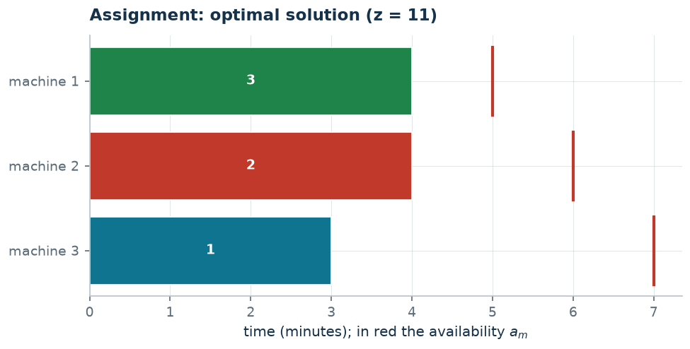
Solution \(\bar x_{13} = \bar x_{22} = \bar x_{31} = 1\), value \(2 + 4 + 5 = 11\): \(\mathit{UB} = 11\), i.e.\ \(z(\mathit{MILP}) \le 11\). Next-fit and first-fit both find \(x_{11} = x_{21} = x_{32} = 1\), of value \(14\).
LP relaxation and dual: the dual bound
The LP relaxation replaces \(x_{jm} \in \{0,1\}\) with \(x_{jm} \ge 0\) (the constraint \(x_{jm} \le 1\) is implied by the assignment constraints). With a free dual variable \(\mu_j\) for each assignment constraint and a non-positive \(\pi_m\) for each availability constraint (\(\le\) in a minimisation), the dual is:
The same dual, written on the data of the instance:
A hand-built dual solution. With \(\bar\pi_m = 0\), the constraints become \(\mu_j \le c_{jm}\) for every \(m\): the largest feasible value is
with value \(10\). By weak duality
The recipe has a meaning: "every job costs at least its minimum cost" is a lower bound anyone would write down; the dual formalises it and says how to improve it, with \(\pi_m < 0\) where the availability is tight.
What the solver says. \(z(\mathit{LP}) = 53/5 = 10.6\) (equal to the optimum of the dual: strong duality), with duals \(\tilde\mu = (2,\ 4.8,\ 5)\) and \(\tilde\pi = (0,\ -0.2,\ 0)\): machine 2 is the tight resource. The integer optimum is \(z(\mathit{MILP}) = 11\) with \(\tilde x_{13} = \tilde x_{22} = \tilde x_{31} = 1\): the best-fit heuristic had found the optimum, but only the solver certifies it — the dual bound stopped at \(10\) (and since the costs are integer, \(\lceil 53/5 \rceil = 11\) closes the gap).
| \(UB\) (best-fit) | \(LB\) (hand dual) | \(z(\mathit{LP})\) | \(z(\mathit{MILP})\) | heuristic gap |
|---|---|---|---|---|
| 11 | 10 | \(53/5\) | 11 | \(0.0\%\) |
Additional considerations
- \(x_{jm} \le 1\) (\(n\,k\) inequalities) are valid but implied by the assignment constraints: they do not strengthen the relaxation (indeed \(z(\mathit{LP}) = z(\mathit{LP}^+)\)).
- If a job \(j\) does not fit on a machine \(m\) (\(t_{jm} > a_m\)), \(x_{jm}\) can be fixed to zero before solving: the model is smaller and the relaxation does not get worse.
Additional modelling questions
7.1.1 — Fixed cost per used machine
Every machine that processes at least one job costs an extra \(g_m = 3\) euros to switch on. Model the fixed cost and find the new optimum. Which link comes into play?
A worked variant: jobs 1 and 3 on the same machine
Jobs 1 and 3 use the same tool and must be processed by the same machine.
It is a link between two variables of the same family: for every machine \(m\), \(x_{1m} = 1\) if and only if \(x_{3m} = 1\), that is
(\(k\) linear constraints). Both directions are imposed by the constraint: if \(x_{1m} = 1\) then \(x_{3m} = 1\) and vice versa; constraints then guarantee that the common machine is unique. On the instance the new optimum is \(12\): the pair must go where \(t_{1m} + t_{3m} \le a_m\), i.e. on machine 1 (\(2 + 4 \le 5\)? no), on machine 2 (\(1 + 5 \le 6\): yes, cost \(10 + 4\)) or on machine 3 (\(3 + 3 \le 7\): yes, cost \(2 + 6\)); with job 2 on machine 2 (\(4\)) the best choice is machine 3 for the pair: \(2 + 6 + 4 = 12\).
The constraint "jobs 1 and 3 on the same machine" adds one free variable \(\sigma_m\) per machine to the dual, and with it the two jobs can be priced together: the constraints of their columns give \(\mu_1 + \mu_3 \le \min_m (c_{1m} + c_{3m})\), which is more than pricing them separately. The heuristic tries the pair on every machine that can hold it and places job 2 last; the two bounds meet and the problem closes without the solver.
| value | what it is | |
|---|---|---|
| \(\mathit{UB}\) | \(12\) | heuristic solution |
| \(\mathit{LB}\) | \(12\) | dual certificate built by hand |
| \(z(\mathit{LP})\) | \(12\) | relaxation without the bounds |
| \(z(\mathit{LP}^+)\) | \(12\) | relaxation with the bounds |
| \(z(\mathit{MILP})\) | \(12\) | optimum of the MILP |
Code
The complete script of the problem — data, model, heuristics, dual,
solution, variants and figures — is
python/fam07_1_assignment.py
(reproducible with python3 python/fam07_1_assignment.py from the python/
folder). The same code is also available as a notebook —
notebooks/fam07_1_assignment.ipynb
— which opens in Colab from the badge at the top of the page.
Show the complete script — python/fam07_1_assignment.py (227 lines)
"""Problem 7.1 -- Minimum-cost assignment with availability (GAP).

A BIP model with a single family of variables: no link to prove, only an
assignment constraint and a per-machine capacity constraint. Next/first/
best-fit heuristics for the upper bound, dual of the LP relaxation with a
hand-built solution for the lower bound.
"""
import gurobipy as gp
import numpy as np
import pandas as pd
from gurobipy import GRB

from euristiche import best_fit, first_fit, matrice, next_fit
from mip import (ammissibile, dualita_forte, due_rilassamenti, frazione,
                 nuovo_modello, registra_bound, rilassamenti, risolvi,
                 stampa_soluzione, valuta)
from stile import CICLO, ROSSO, intestazione, plt, salva_dati, salva_figura
from esteso import salva_modello

R = range

# ---------- 1. MODEL AND INSTANCE ----------
intestazione("1. Minimum-cost assignment: n jobs, k machines, availability a_m")
t1 = [[2, 1, 3], [3, 4, 2], [4, 5, 3]]
c1 = [[5, 10, 2], [5, 4, 6], [5, 4, 6]]
a1 = [5, 6, 7]
n, k = 3, 3
salva_dati(pd.DataFrame([{"job": j + 1, "machine": m + 1, "t": t1[j][m], "c": c1[j][m]}
                         for j in R(n) for m in R(k)]), "fam07_1_lavori")
salva_dati(pd.DataFrame({"machine": R(1, k + 1), "a": a1}), "fam07_1_macchine")


def modello_1(t, c, a):
    n, k = len(t), len(a)
    m = nuovo_modello("assegnamento")
    x = m.addVars(n, k, vtype=GRB.BINARY, name="x")
    m.setObjective(gp.quicksum(c[j][mm] * x[j, mm] for j in R(n) for mm in R(k)), GRB.MINIMIZE)
    m.addConstrs((x.sum(j, "*") == 1 for j in R(n)), name="assegna")
    m.addConstrs((gp.quicksum(t[j][mm] * x[j, mm] for j in R(n)) <= a[mm] for mm in R(k)),
                 name="disponibilita")
    return m, x


def duale_1(t, c, a):
    """Dual of the LP relaxation: max sum mu_j + sum a_m pi_m, mu_j + t_jm pi_m <= c_jm, pi <= 0."""
    n, k = len(t), len(a)
    d = nuovo_modello("duale_assegnamento")
    mu = d.addVars(n, lb=-GRB.INFINITY, name="mu")
    pi = d.addVars(k, lb=-GRB.INFINITY, ub=0.0, name="pi")
    d.setObjective(mu.sum() + gp.quicksum(a[mm] * pi[mm] for mm in R(k)), GRB.MAXIMIZE)
    d.addConstrs((mu[j] + t[j][mm] * pi[mm] <= c[j][mm] for j in R(n) for mm in R(k)), name="rc")
    return d


def valore_1(e, c):
    return sum(c[j][mm] for (j, mm) in e.x)


m1, x1 = modello_1(t1, c1, a1)
salva_modello(m1, "fam07_1_primale")

# ---------- 2. THE LP RELAXATION ----------
zlp1, zlp1r, pi_lp = rilassamenti(m1)
print("Duals of the relaxation read from Gurobi:", {kk: round(v, 4) for kk, v in pi_lp.items()})

# ---------- 3. THE DUAL OF THE RELAXATION (LOWER BOUND) ----------
d1 = duale_1(t1, c1, a1)
salva_modello(d1, "fam07_1_duale")
mano = {f"mu[{j}]": min(c1[j]) for j in R(n)}
lb1, viol = valuta(d1, mano)
assert viol <= 1e-9, viol
print(f"Hand-built dual solution: pi = 0, mu_j = min_m c_jm = "
      + ", ".join(frazione(mano[f"mu[{j}]"]) for j in R(n)) + f"  ->  lb = {frazione(lb1)}")
dualita_forte(d1, zlp1)

# ---------- 4. CONSTRUCTIVE HEURISTIC (UPPER BOUND) ----------
print("Constructive heuristics:")
e_next = next_fit(t1, a1)
e_first = first_fit(t1, a1)
e_best = best_fit(t1, a1, lambda j, mm, ra: c1[j][mm], "cost")
for nome, e in [("next-fit", e_next), ("first-fit", e_first), ("best-fit (minimum cost)", e_best)]:
    print(f"  {nome:26s} ub = {valore_1(e, c1)}   assignment "
          + ", ".join(f"x[{j + 1}][{mm + 1}]" for (j, mm) in sorted(e.x)))
print("Step-by-step run of the best-fit:")
e_best.traccia.stampa()
ub1 = valore_1(e_best, c1)
sol_eur = {f"x[{j},{mm}]": 1 for (j, mm) in e_best.x}
assert ammissibile(m1, sol_eur)

# ---------- 5. OPTIMAL SOLUTION OF THE MILP ----------
z1 = risolvi(m1)
print("Optimal solution of the MILP:")
stampa_soluzione(m1, solo_non_nulle=True)
riga = registra_bound("1 assignment", ub1, lb1, zlp1, zlp1r, z1)
salva_dati(pd.DataFrame([riga]), "fam07_1_bound")
ott1 = {(j, mm) for j in R(n) for mm in R(k) if x1[j, mm].X > 0.5}

# ---------- 6. ADDITIONAL MODELLING QUESTIONS ----------


varianti = {}


def variante(nome, m):
    z = risolvi(m)
    print(f"  {nome:70s} z = {frazione(z)}")
    return z

# 1a: jobs 1 and 3 must be on the same machine
m, x = modello_1(t1, c1, a1)
m.addConstrs((x[0, mm] == x[2, mm] for mm in R(3)), name="together")
varianti["1a"] = variante("1a. Jobs 1 and 3 on the same machine (x_1m = x_3m)", m)
# 1b: fixed cost g_m per used machine (activation)
g1 = [3, 3, 3]
m, x = modello_1(t1, c1, a1)
y = m.addVars(3, vtype=GRB.BINARY, name="y")
m.addConstrs((x[j, mm] <= y[mm] for j in R(3) for mm in R(3)), name="activate")
m.update()
m.setObjective(m.getObjective() + gp.quicksum(g1[mm] * y[mm] for mm in R(3)), GRB.MINIMIZE)
varianti["1b"] = variante("1b. Fixed cost g_m = 3 per used machine (x_jm <= y_m)", m)
salva_dati(pd.DataFrame({"variant": list(varianti), "z": list(varianti.values())}), "fam07_1_varianti")

# ---------- 7. THE SANDWICH ON THE VARIANT 1a ----------
# A variant does not merely change the optimum: it changes both bounds too, and the
# dual bound is built with the same recipe as the base problem, enriched by the
# new dual family.
intestazione("1a. The sandwich on the variant: jobs 1 and 3 on the same machine")


def modello_1a(t, c, a):
    """Model 7.1 with the constraint x_1m = x_3m for every machine."""
    mm_, xx = modello_1(t, c, a)
    mm_.addConstrs((xx[0, mz] - xx[2, mz] == 0 for mz in R(len(a))), name="insieme")
    return mm_, xx


def duale_1a(t, c, a):
    """Dual of the relaxation: to the dual of 7.1 one free variable sigma_m is
    added for each equality x_1m - x_3m = 0. The columns of jobs 1 and 3 see
    it with opposite signs."""
    nn, kk = len(t), len(a)
    d = nuovo_modello("duale_assegnamento_1a")
    mu = d.addVars(nn, lb=-GRB.INFINITY, name="mu")
    pi = d.addVars(kk, lb=-GRB.INFINITY, ub=0.0, name="pi")
    sg = d.addVars(kk, lb=-GRB.INFINITY, name="sigma")
    d.setObjective(mu.sum() + gp.quicksum(a[mz] * pi[mz] for mz in R(kk)), GRB.MAXIMIZE)
    for mz in R(kk):
        d.addConstr(mu[0] + t[0][mz] * pi[mz] + sg[mz] <= c[0][mz], name=f"rc0{mz}")
        d.addConstr(mu[1] + t[1][mz] * pi[mz] <= c[1][mz], name=f"rc1{mz}")
        d.addConstr(mu[2] + t[2][mz] * pi[mz] - sg[mz] <= c[2][mz], name=f"rc2{mz}")
    return d


m1a, x1a = modello_1a(t1, c1, a1)
salva_modello(m1a, "fam07_1a_primale")

# -- feasible heuristic: pick the machine of the pair, then the rest --
print("Constructive heuristic: the pair (1, 3) is tried on every machine that can")
print("hold it, then job 2 goes to the cheapest machine among those with room.")
migliore = None
for mz in R(k):
    if t1[0][mz] + t1[2][mz] > a1[mz]:
        print(f"  pair on machine {mz + 1}: it needs "
              f"{t1[0][mz] + t1[2][mz]} minutes out of {a1[mz]} -> it does not fit")
        continue
    residuo = [a1[q] - (t1[0][mz] + t1[2][mz] if q == mz else 0) for q in R(k)]
    capienti = [q for q in R(k) if t1[1][q] <= residuo[q]]
    if not capienti:
        print(f"  pair on machine {mz + 1}: job 2 does not fit anywhere")
        continue
    scelta = min(capienti, key=lambda q: c1[1][q])
    valore = c1[0][mz] + c1[2][mz] + c1[1][scelta]
    print(f"  pair on machine {mz + 1} (cost {c1[0][mz] + c1[2][mz]}), "
          f"job 2 on machine {scelta + 1} (cost {c1[1][scelta]})  ->  {valore}")
    if migliore is None or valore < migliore[0]:
        migliore = (valore, mz, scelta)
ub1a, mz_coppia, mz_due = migliore
sol_1a = {f"x[0,{mz_coppia}]": 1, f"x[2,{mz_coppia}]": 1, f"x[1,{mz_due}]": 1}
assert ammissibile(m1a, sol_1a), "the heuristic solution of the variant must be feasible"
print(f"  ub = {frazione(ub1a)}")

# -- dual certificate: the pair lets jobs 1 and 3 be priced together --
d1a = duale_1a(t1, c1, a1)
salva_modello(d1a, "fam07_1a_duale")
coppia = min(c1[0][mz] + c1[2][mz] for mz in R(k))
mano_1a = {"mu[0]": min(c1[0]), "mu[1]": min(c1[1]), "mu[2]": coppia - min(c1[0])}
mano_1a.update({f"sigma[{mz}]": c1[0][mz] - min(c1[0]) for mz in R(k)})
lb1a, viol_1a = valuta(d1a, mano_1a)
assert viol_1a <= 1e-9, viol_1a
print("Dual solution by hand: pi = 0; the constraints of columns 1 and 3 give")
print(f"  mu_1 + mu_3 <= min_m (c_1m + c_3m) = {frazione(coppia)}, that is, the two jobs")
print("  are priced together because they travel together. One sets mu_1 = min_m c_1m,")
print("  mu_3 = the difference, sigma_m = c_1m - mu_1, and mu_2 = min_m c_2m.")
print(f"  ->  lb = {frazione(lb1a)}   (the recipe of the base problem would give "
      f"{frazione(sum(min(c1[j]) for j in R(n)))}: the pair is worth more)")
zlp1a, zlp1ar, _ = due_rilassamenti(m1a, d1a)
z1a = risolvi(m1a)
riga_1a = registra_bound("1a jobs 1 and 3 together", ub1a, lb1a, zlp1a, zlp1ar, z1a)
salva_dati(pd.DataFrame([riga_1a]), "fam07_1a_bound")
assert lb1a <= zlp1a <= z1a <= ub1a + 1e-9

# ---------- 8. FIGURES ----------


def barre_macchine(assegn, t, a, titolo, nome):
    """Every machine: bar of the times of the assigned jobs and availability."""
    k = len(a)
    fig, ax = plt.subplots(figsize=(7.2, 3.2))
    for mm in R(k):
        inizio = 0
        for (j, m2) in sorted(assegn):
            if m2 == mm:
                ax.barh(mm, t[j][mm], left=inizio, color=CICLO[j % len(CICLO)], edgecolor="white")
                ax.text(inizio + t[j][mm] / 2, mm, f"{j + 1}", ha="center", va="center", color="white",
                        fontsize=9, fontweight="bold")
                inizio += t[j][mm]
        ax.plot([a[mm], a[mm]], [mm - 0.4, mm + 0.4], color=ROSSO, lw=2)
    ax.set_yticks(R(k))
    ax.set_yticklabels([f"machine {mm + 1}" for mm in R(k)])
    ax.set_xlabel("time (minutes); in red the availability $a_m$")
    ax.set_title(titolo)
    ax.invert_yaxis()
    salva_figura(fig, nome)

barre_macchine(e_best.x, t1, a1, "Assignment: best-fit solution (ub = 11)", "cap07_gap_euristica")
barre_macchine(ott1, t1, a1, f"Assignment: optimal solution (z = {frazione(z1)})", "cap07_gap_ottimo")
print("Done.")