Machines with a fixed usage cost
Class: BIP · Links: activation (aggregated) · Script: python/fam07_2_fixedcost.py
Difficulty: ★★☆☆☆ · Time: 30–45 min

Problem 7.2
A company needs to process \(n \in \mathbb{Z}_{\ge 1}\) jobs and has \(k \in \mathbb{Z}_{\ge 1}\) machines. For each job \(j \in \{1, 2, \dots, n\}\) and each machine \(m \in \{1, 2, \dots, k\}\), the value \(t_{jm} \in \mathbb{Q}_{>0}\) is the processing time in minutes. For each machine \(m\), the value \(a_m \in \mathbb{Q}_{>0}\) is the availability in minutes and the value \(c_m \in \mathbb{Q}_{>0}\) is the cost in euros if the machine is used. Each machine processes one job at a time. The company wants to assign all jobs minimising the cost of the machines used.
The problem in words. We decide which machines to switch on and on which machine each job is processed. The objective: total cost of the machines switched on. The constraints: every job on exactly one machine; a machine switched off processes no job; a machine switched on does not exceed its availability. Compared with problem 7.1 the cost is no longer on the assignments but on the machines: activation variables are needed.
Model
Data (input of the model).
| Symbol | Type | Meaning |
|---|---|---|
| \(n\) | \(\in \mathbb{Z}_{\ge 1}\) | number of jobs, \(j \in \{1, 2, \dots, n\}\) |
| \(k\) | \(\in \mathbb{Z}_{\ge 1}\) | number of machines, \(m \in \{1, 2, \dots, k\}\) |
| \(t_{jm}\) | \(\in \mathbb{Q}_{>0}\) | processing time of job \(j\) on machine \(m\) |
| \(a_m\) | \(\in \mathbb{Q}_{>0}\) | availability of machine \(m\) |
| \(c_m\) | \(\in \mathbb{Q}_{>0}\) | fixed cost if machine \(m\) is used |
Decision variables. We introduce the following \(n\,k + k\) binary variables:
- the objective minimises the total cost of the machines used;
- the assignment constraints ensure that each job is assigned to exactly one machine (\(n\) linear constraints);
- the link constraints connect assignments and usage and impose the capacity restrictions: if at least one job is assigned to a machine then the machine is used, no job is assigned to an unused machine and, if the machine is used, the total processing time does not exceed its availability (\(k\) linear constraints);
- the domain constraints define the variables.
Link between the variables
Imposed by the constraint. For each machine \(m\), if the total processing time of the jobs assigned to it is positive, the machine must be used:
The link constraint gives \(\sum_j t_{jm} x_{jm} \le a_m y_m\): if the left-hand side is positive then \(a_m y_m > 0\), hence \(y_m > 0\) and, being binary, \(y_m = 1\). Conversely, if \(y_m = 0\) then \(\sum_j t_{jm} x_{jm} \le 0\) and, with \(t_{jm} > 0\) and \(x_{jm} \ge 0\), all the \(x_{jm}\) are zero.
Imposed by the optimum. Conversely, if the total processing time is zero the machine is not used: \(\sum_j t_{jm} x_{jm} = 0 \Longrightarrow y_m = 0\) (contrapositive: \(y_m = 1 \Longrightarrow\) at least one job assigned). This is not imposed by the constraints (\(y_m = 1\) with no jobs is feasible), but it follows from the objective in every optimum: since \(c_m > 0\), if \(y_m = 1\) with no jobs, setting \(y_m = 0\) keeps the constraints (\(0 \ge 0\)) and reduces the cost by \(c_m\).
The model in gurobipy
m = gp.Model("fixed_cost");  m.Params.OutputFlag = 0
x = m.addVars(n, k, vtype=GRB.BINARY, name="x")
y = m.addVars(k, vtype=GRB.BINARY, name="y")
m.setObjective(gp.quicksum(c[mm] * y[mm] for mm in range(k)), GRB.MINIMIZE)
m.addConstrs((x.sum(j, "*") == 1 for j in range(n)), name="assign")
m.addConstrs((-gp.quicksum(t[j][mm] * x[j, mm] for j in range(n))
              + a[mm] * y[mm] >= 0 for mm in range(k)), name="link")
m.optimize()
The instance
\(n = 3\) jobs, \(k = 3\) machines:
| \(t_{jm}\) | \(m=1\) | \(m=2\) | \(m=3\) |
|---|---|---|---|
| \(j=1\) | 6 | 5 | 3 |
| \(j=2\) | 5 | 10 | 2 |
| \(j=3\) | 20 | 13 | 10 |
| \(m=1\) | \(m=2\) | \(m=3\) | |
|---|---|---|---|
| \(c_m\) | 8 | 7 | 5 |
| \(a_m\) | 25 | 20 | 12 |
The model for the instance: objective \(\min\ 8y_1 + 7y_2 + 5y_3\); three assignment constraints; the three link constraints \(-6x_{11} - 5x_{21} - 20x_{31} + 25y_1 \ge 0\), \(-5x_{12} - 10x_{22} - 13x_{32} + 20y_2 \ge 0\), \(-3x_{13} - 2x_{23} - 10x_{33} + 12y_3 \ge 0\).
The model written on the data of the instance:
Constructive heuristic: the primal bound
The best-fit criterion becomes the minimum time (there are no assignment costs: it pays to consume little availability).
- Step 1. Job 1: \(ra = (25, 20, 12)\); times \(6, 5, 3\): minimum on machine 3, \(x[1][3] = 1\), \(ra[3] = 9\).
- Step 2. Job 2: times \(5, 10, 2\): minimum on machine 3, \(x[2][3] = 1\), \(ra[3] = 7\).
- Step 3. Job 3: machine 3 is not enough (\(10 > 7\)); between \(20\) and \(13\) the minimum is machine 2, \(x[3][2] = 1\), \(ra[2] = 7\).
Machines used: 2 and 3: \(\bar y = (0, 1, 1)\), value \(12\), hence \(z(\mathit{MILP}) \le 12\). Next-fit, first-fit and the "opened machines first" variants use machines 1 and 2 (value \(15\)).
LP relaxation and dual: the dual bound
With \(\mu_j\) free (assignment) and \(\pi_m \ge 0\) (link, \(\ge\) in a minimisation):
The same dual, written on the data of the instance:
A hand-built dual solution. \(\bar\pi_m = c_m / a_m\) (the cost per minute of each machine): \(\tfrac{8}{25}, \tfrac{7}{20}, \tfrac{5}{12}\); then \(\bar\mu_j = \min_m t_{jm}\bar\pi_m\): \(\bar\mu_1 = \min\{\tfrac{48}{25}, \tfrac{7}{4}, \tfrac{5}{4}\} = \tfrac{5}{4}\), \(\bar\mu_2 = \min\{\tfrac{8}{5}, \tfrac{7}{2}, \tfrac{5}{6}\} = \tfrac{5}{6}\), \(\bar\mu_3 = \min\{\tfrac{32}{5}, \tfrac{91}{20}, \tfrac{25}{6}\} = \tfrac{25}{6}\). Value \(\tfrac{25}{4}\):
A weak bound: the fixed cost of a machine is paid in full as soon as it is used, but the relaxation spreads it over the minutes.
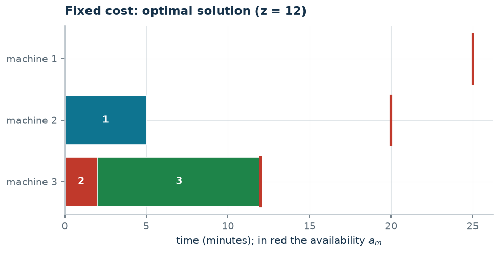
What the solver says. \(z(\mathit{LP}) = 25/4\): the hand-built solution is optimal for the dual. With \(y_m \le 1\) and \(x_{jm} \le 1\) the strengthened relaxation is \(z(\mathit{LP}^+) = 1273/200 = 6.365\); with the disaggregated links \(x_{jm} \le y_m\) it rises to \(440/67 = 6.567\). Integer optimum \(12\): machines 2 and 3 on, \(\tilde x_{12} = \tilde x_{23} = \tilde x_{33} = 1\).
| \(UB\) | \(LB\) (hand dual) | \(z(\mathit{LP})\) | \(z(\mathit{LP}^+)\) | \(z(\mathit{MILP})\) | heuristic gap |
|---|---|---|---|---|---|
| 12 | \(25/4\) | \(25/4\) | \(1273/200\) | 12 | \(0.0\%\) |
Additional considerations
- \(y_m \le 1\) and \(x_{jm} \le 1\) are valid; the former strengthen the relaxation (\(6.25 \to 6.365\)).
- "If at least one job is assigned to \(m\) then \(m\) is used" is \((x_{1m} \,\mathtt{OR}\, \dots \,\mathtt{OR}\, x_{nm}) \Rightarrow y_m\); De Morgan and distributivity give the CNF \((\mathtt{NOT}\,x_{1m} \,\mathtt{OR}\, y_m) \,\mathtt{AND}\, \dots\), i.e.\ the disaggregated constraints \(x_{jm} \le y_m\): implied by the model, but not by the relaxation — added, they bring \(z(\mathit{LP}^+)\) to \(440/67\). Same set of integer solutions, tighter relaxation.
- The opposite direction, \(\sum_j x_{jm} \ge y_m\), is not valid but can be added without losing the optimum.
Additional modelling questions
7.2.1 — Minimum usage of a machine switched on
Every machine used must work at least \(\ell = 8\) minutes. Model and find the new optimum.
A worked variant: link between two activations
Machine 3 shares the power supply with machine 1: if machine 1 is used, machine 3 must be used too.
It is an implication between two binary variables, \(y_1 \Longrightarrow y_3\), i.e. \(\NOT y_1 \OR y_3\), already in CNF: the linear constraint is
(one linear constraint). It imposes that \(y_1 = 1\) forces \(y_3 = 1\) and, by contraposition, that \(y_3 = 0\) forces \(y_1 = 0\). It does not impose the converse: machine 3 can be used alone (\(y_3 = 1\), \(y_1 = 0\) is feasible), and \(y_1 = y_3 = 0\) stays feasible. On the instance the constraint does not change the optimum, \(12\), because the optimal solution does not use machine 1; it would change it if the costs made machine 1 alone convenient.
The link "if machine 1 is used then machine 3 is used too" adds a variable \(\rho \le 0\) to the dual, which loosens the column of \(y_1\) and tightens that of \(y_3\). On the data of the instance it does not pay to move it: machine 3 is the minimum for every job, and lowering its price would lower every \(\mu_j\). The certificate stays the one of the base problem — a link between activations does not touch the relaxation, which can switch on half a machine. What grows is the integer optimum, and therefore the gap.
| value | what it is | |
|---|---|---|
| \(\mathit{UB}\) | \(12\) | heuristic solution |
| \(\mathit{LB}\) | \(\frac{25}{4}\) | dual certificate built by hand |
| \(z(\mathit{LP})\) | \(\frac{25}{4}\) | relaxation without the bounds |
| \(z(\mathit{LP}^+)\) | \(\frac{1273}{200}\) | relaxation with the bounds |
| \(z(\mathit{MILP})\) | \(12\) | optimum of the MILP |
Code
Full script: python/fam07_2_fixedcost.py;
notebook: notebooks/fam07_2_fixedcost.ipynb.
Show the complete script — python/fam07_2_fixedcost.py (218 lines)
"""Problem 7.2 -- Machines with a fixed usage cost.

The activation variables y_m are born here: the link with the assignment
variables x_jm is proved in both directions (one imposed by the constraint,
the other by the optimum). Comparison between aggregated and disaggregated
relaxation.
"""
import gurobipy as gp
import numpy as np
import pandas as pd
from gurobipy import GRB

from euristiche import best_fit, first_fit, matrice, next_fit
from mip import (ammissibile, dualita_forte, due_rilassamenti, frazione,
                 nuovo_modello, registra_bound, rilassamenti, rilassamento, risolvi,
                 stampa_soluzione, valuta)
from stile import CICLO, ROSSO, intestazione, plt, salva_dati, salva_figura
from esteso import salva_modello

R = range

# ---------- 1. MODEL AND INSTANCE ----------
intestazione("2. Fixed cost per used machine: activation variables y_m")
t2 = [[6, 5, 3], [5, 10, 2], [20, 13, 10]]
c2 = [8, 7, 5]
a2 = [25, 20, 12]
salva_dati(pd.DataFrame([{"job": j + 1, "machine": m + 1, "t": t2[j][m]}
                         for j in R(3) for m in R(3)]), "fam07_2_lavori")
salva_dati(pd.DataFrame({"machine": R(1, 4), "c": c2, "a": a2}), "fam07_2_macchine")


def modello_2(t, c, a):
    n, k = len(t), len(a)
    m = nuovo_modello("costo_fisso")
    x = m.addVars(n, k, vtype=GRB.BINARY, name="x")
    y = m.addVars(k, vtype=GRB.BINARY, name="y")
    m.setObjective(gp.quicksum(c[mm] * y[mm] for mm in R(k)), GRB.MINIMIZE)
    m.addConstrs((x.sum(j, "*") == 1 for j in R(n)), name="assegna")
    m.addConstrs((-gp.quicksum(t[j][mm] * x[j, mm] for j in R(n)) + a[mm] * y[mm] >= 0
                  for mm in R(k)), name="link")
    return m, x, y


def duale_2(t, c, a):
    """max sum mu_j;  mu_j - t_jm pi_m <= 0;  a_m pi_m <= c_m;  pi >= 0, mu libere."""
    n, k = len(t), len(a)
    d = nuovo_modello("duale_costo_fisso")
    mu = d.addVars(n, lb=-GRB.INFINITY, name="mu")
    pi = d.addVars(k, name="pi")
    d.setObjective(mu.sum(), GRB.MAXIMIZE)
    d.addConstrs((mu[j] - t[j][mm] * pi[mm] <= 0 for j in R(n) for mm in R(k)), name="rc_x")
    d.addConstrs((a[mm] * pi[mm] <= c[mm] for mm in R(k)), name="rc_y")
    return d


def valore_2(e, c):
    return sum(c[mm] * y for mm, y in enumerate(e.y))


m2, x2, y2 = modello_2(t2, c2, a2)
salva_modello(m2, "fam07_2_primale")

# ---------- 2. THE LP RELAXATION ----------
zlp2, zlp2r, _ = rilassamenti(m2)

# ---------- 3. THE DUAL OF THE RELAXATION (LOWER BOUND) ----------
d2 = duale_2(t2, c2, a2)
salva_modello(d2, "fam07_2_duale")
mano = {f"pi[{mm}]": c2[mm] / a2[mm] for mm in R(3)}
mano.update({f"mu[{j}]": min(t2[j][mm] * c2[mm] / a2[mm] for mm in R(3)) for j in R(3)})
lb2, viol = valuta(d2, mano)
assert viol <= 1e-9
print("Hand-built dual solution: pi_m = c_m/a_m = " + ", ".join(frazione(c2[mm] / a2[mm]) for mm in R(3))
      + ";  mu_j = min_m t_jm pi_m = " + ", ".join(frazione(mano[f"mu[{j}]"]) for j in R(3))
      + f"  ->  lb = {frazione(lb2)}")
dualita_forte(d2, zlp2)

# ---------- 4. CONSTRUCTIVE HEURISTIC (UPPER BOUND) ----------
print("Constructive heuristics:")
eur2 = [("next-fit", next_fit(t2, a2)),
        ("first-fit", first_fit(t2, a2)),
        ("best-fit (minimum time)", best_fit(t2, a2, lambda j, mm, ra: t2[j][mm], "time")),
        ("first-fit on opened machines", first_fit(t2, a2, solo_aperte=True)),
        ("best-fit on opened (tightest fit)", best_fit(t2, a2, lambda j, mm, ra: ra[mm] - t2[j][mm],
                                                      "slack", solo_aperte=True))]
for nome, e in eur2:
    print(f"  {nome:34s} ub = {valore_2(e, c2):3d}   machines used "
          + str([mm + 1 for mm, y in enumerate(e.y) if y]))
print("Step-by-step run of the minimum-time best-fit:")
eur2[2][1].traccia.stampa()
ub2 = min(valore_2(e, c2) for _, e in eur2)

# ---------- 5. OPTIMAL SOLUTION OF THE MILP ----------
z2 = risolvi(m2)
print("Optimal solution of the MILP:")
stampa_soluzione(m2, solo_non_nulle=True)
riga = registra_bound("2 fixed cost", ub2, lb2, zlp2, zlp2r, z2)
salva_dati(pd.DataFrame([riga]), "fam07_2_bound")

# ---------- 6. RELAXATION WITH THE DISAGGREGATED LINKS ----------
# the same instance with the disaggregated link constraints x_jm <= y_m: stronger relaxation
m2d, x2d, y2d = modello_2(t2, c2, a2)
m2d.addConstrs((x2d[j, mm] <= y2d[mm] for j in R(3) for mm in R(3)), name="disaggregated")
zlp2d, _, _ = rilassamento(m2d, rafforzato=True)
print(f"Relaxation with the bounds with the disaggregated links x_jm <= y_m: z(LP+) = {frazione(zlp2d)} "
      f"(with the aggregated link only: {frazione(zlp2r)}) — the disaggregated formulation is stronger")

# ---------- 7. ADDITIONAL MODELLING QUESTIONS ----------


varianti = {}


def variante(nome, m):
    z = risolvi(m)
    print(f"  {nome:70s} z = {frazione(z)}")
    return z

# 2a: a used machine must work at least 8 minutes (link in the opposite direction)
m, x, y = modello_2(t2, c2, a2)
m.addConstrs((gp.quicksum(t2[j][mm] * x[j, mm] for j in R(3)) >= 8 * y[mm] for mm in R(3)), name="min_usage")
varianti["2a"] = variante("2a. A used machine works at least 8 minutes (sum_j t_jm x_jm >= 8 y_m)", m)
# 2b: if machine 1 is used then machine 3 is used too (link between activations)
m, x, y = modello_2(t2, c2, a2)
m.addConstr(y[0] <= y[2], name="1_implies_3")
varianti["2b"] = variante("2b. If machine 1 is used so is machine 3 (y_1 <= y_3)", m)
salva_dati(pd.DataFrame({"variant": list(varianti), "z": list(varianti.values())}), "fam07_2_varianti")

# ---------- 8. THE SANDWICH ON THE VARIANT 2b ----------
intestazione("2b. The sandwich on the variant: if machine 1 is used then machine 3 is used too")


def modello_2b(t, c, a):
    mm_, xx, yy = modello_2(t, c, a)
    mm_.addConstr(yy[0] - yy[2] <= 0, name="1_implica_3")
    return mm_, xx, yy


def duale_2b(t, c, a):
    """To the dual of 7.2 one adds rho <= 0 for the constraint y_1 - y_3 <= 0: it
    appears in the column of y_1 with a plus sign and in that of y_3 with a
    minus sign. The right-hand side is zero, so the objective does not change."""
    nn, kk = len(t), len(a)
    d = nuovo_modello("duale_costo_fisso_2b")
    mu = d.addVars(nn, lb=-GRB.INFINITY, name="mu")
    pi = d.addVars(kk, name="pi")
    rho = d.addVar(lb=-GRB.INFINITY, ub=0.0, name="rho")
    d.setObjective(mu.sum(), GRB.MAXIMIZE)
    d.addConstrs((mu[j] - t[j][mz] * pi[mz] <= 0 for j in R(nn) for mz in R(kk)), name="rc_x")
    d.addConstr(a[0] * pi[0] + rho <= c[0], name="rc_y0")
    d.addConstr(a[1] * pi[1] <= c[1], name="rc_y1")
    d.addConstr(a[2] * pi[2] - rho <= c[2], name="rc_y2")
    return d


m2b, x2b, y2b = modello_2b(t2, c2, a2)
salva_modello(m2b, "fam07_2b_primale")

# -- feasible heuristic: the base one, repaired --
print("Constructive heuristic: start from the solution of the base problem and, if it uses")
print("machine 1 without machine 3, switch machine 3 on as well (a repair of known cost).")
e_base2 = min((e for _, e in eur2), key=lambda e: valore_2(e, c2))
usate = sorted({mz for (_, mz) in e_base2.x})
print(f"  base solution: machines used {[mz + 1 for mz in usate]}, cost "
      f"{frazione(sum(c2[mz] for mz in usate))}")
usate_b = sorted(set(usate) | ({2} if 0 in usate else set()))
ub2b = sum(c2[mz] for mz in usate_b)
sol_2b = {f"x[{j},{mz}]": 1 for (j, mz) in e_base2.x} | {f"y[{mz}]": 1 for mz in usate_b}
assert ammissibile(m2b, sol_2b), "the heuristic solution of the variant must be feasible"
print(f"  after the repair: machines {[mz + 1 for mz in usate_b]}  ->  ub = {frazione(ub2b)}")

# -- dual certificate --
d2b = duale_2b(t2, c2, a2)
salva_modello(d2b, "fam07_2b_duale")
mano_2b = {f"pi[{mz}]": c2[mz] / a2[mz] for mz in R(3)}
mano_2b.update({f"mu[{j}]": min(t2[j][mz] * mano_2b[f"pi[{mz}]"] for mz in R(3)) for j in R(3)})
mano_2b["rho"] = 0.0
lb2b, viol_2b = valuta(d2b, mano_2b)
assert viol_2b <= 1e-9, viol_2b
print("Dual solution by hand: rho = 0 and the recipe of the base problem, pi_m = c_m / a_m,")
print("  mu_j = min_m t_jm pi_m. Raising pi_1 at the expense of pi_3 does not pay: machine 3")
print("  is the minimum for all three jobs, so lowering pi_3 lowers every mu_j.")
print(f"  ->  lb = {frazione(lb2b)}")
zlp2b, zlp2br, _ = due_rilassamenti(m2b, d2b)
z2b = risolvi(m2b)
riga_2b = registra_bound("2b machine 1 implies machine 3", ub2b, lb2b, zlp2b, zlp2br, z2b)
salva_dati(pd.DataFrame([riga_2b]), "fam07_2b_bound")
assert lb2b <= zlp2b <= z2b <= ub2b + 1e-9
print("The certificate does not move from the base problem: a link between activations")
print("does not touch the relaxation, because the relaxation can switch on half a machine.")
print("What grows is the integer optimum, and therefore the gap.")

# ---------- 9. FIGURES ----------


def barre_macchine(assegn, t, a, titolo, nome):
    """Every machine: bar of the times of the assigned jobs and availability."""
    k = len(a)
    fig, ax = plt.subplots(figsize=(7.2, 3.2))
    for mm in R(k):
        inizio = 0
        for (j, m2) in sorted(assegn):
            if m2 == mm:
                ax.barh(mm, t[j][mm], left=inizio, color=CICLO[j % len(CICLO)], edgecolor="white")
                ax.text(inizio + t[j][mm] / 2, mm, f"{j + 1}", ha="center", va="center", color="white",
                        fontsize=9, fontweight="bold")
                inizio += t[j][mm]
        ax.plot([a[mm], a[mm]], [mm - 0.4, mm + 0.4], color=ROSSO, lw=2)
    ax.set_yticks(R(k))
    ax.set_yticklabels([f"machine {mm + 1}" for mm in R(k)])
    ax.set_xlabel("time (minutes); in red the availability $a_m$")
    ax.set_title(titolo)
    ax.invert_yaxis()
    salva_figura(fig, nome)

ott2 = {(j, mm) for j in R(3) for mm in R(3) if x2[j, mm].X > 0.5}
barre_macchine(ott2, t2, a2, f"Fixed cost: optimal solution (z = {frazione(z2)})", "cap07_costo_fisso_ottimo")
print("Done.")