1. What is a MIP model
Class: LP · ILP · BIP · MILP · Script: python/cap01_models.py
Data, variables, objective, constraints
A mathematical programming model translates a decision into four ingredients, always in the same order: the data (the numbers known before deciding), the variables (what the decision maker controls), the objective (a function of the variables to minimise or maximise) and the constraints (the equations and inequalities that make a solution feasible).
Notation for optimal values
\(X\) is the feasible set (the points satisfying all constraints, domains included); \(z(\mathit{MILP})\), \(z(\mathit{LP})\), \(z(\mathit{D})\) are the optimal values of the MILP, of its relaxation and of the dual of the relaxation. Feasible solutions carry a bar (\(\bar x\)), optimal ones a tilde (\(\tilde x\)). The bounds are called \(\mathit{LB}\) and \(\mathit{UB}\), whatever the direction of the objective; when the solution they come from matters we write \(\mathit{LB}(\bar x)\), \(\mathit{UB}(\bar x)\) for a feasible solution of the model and \(\mathit{LB}(\bar\pi)\), \(\mathit{UB}(\bar\pi)\) for a feasible solution of the dual. We always write \(z(\mathit{MILP})\) and never \(z^\star\): which model is being optimised must be explicit.
Classes of models. Upright LP is the class of problems, italic \(\mathit{LP}\) is one problem of that class; the same for ILP, BIP and MILP. A model has \(n\) variables, with \(j \in \{1, 2, \dots, n\}\), and \(m\) constraints, with \(i \in \{1, 2, \dots, m\}\); the data are the costs \(c_j\), the coefficients \(a_{ij}\) and the right-hand sides \(b_i\).
What a model can contain:
- a linear objective function of the variables, to be minimised or maximised;
- linear constraints of three types: \(\ge\), for a requirement to be met; \(\le\), for a capacity to be respected; equality, for a balance or an exact assignment;
- variables, in one or more families, each with its own domain, declared at the end of the model.
None of the three has a fixed shape: how many constraints, of which type and with how many families of variables is decided by the problem.
What tells the four classes apart: the domains.
- LP: all the variables continuous. In this course a model of LP type is never written from scratch: it arrives as the relaxation of a MIP model, when the integrality constraints are dropped.
- ILP: all the variables integer.
- BIP: all the variables binary.
- MILP: some integer or binary and others continuous.
That is where the difference in difficulty lives: an LP is solved in polynomial time, an ILP and a MILP in general are not.
A model of ILP type
How many units to buy from two suppliers, \(x_1\) and \(x_2\), in whole lots.
The objective minimises the spending; the \(\ge\) constraint covers the demand of \(12\) units, the \(\le\) one caps the total lots at five. All the variables are integer: it is an ILP.
A model of BIP type
Which projects to fund: \(y_k = 1\) if project \(k\) is funded, \(0\) otherwise.
The objective maximises the value of the projects chosen; the \(\le\) constraint allows at most two of them, the \(\ge\) one requires at least one of the first and the third. All the variables are binary: it is a BIP.
A model of MILP type
Two products to make, with \(x_1\) and \(x_2\) the quantities produced, and a plant to switch on or not, with \(y = 1\) if it is switched on and \(y = 0\) otherwise.
The objective maximises the revenue minus the cost of the plant; the equality requires exactly six units to be produced, the \(\le\) constraint allows at most four units of the second product and only with the plant on (with \(y = 0\) it leaves \(x_2 \le 0\)), the \(\ge\) constraint asks for at least one unit of the first. Two continuous variables and one binary: it is a MILP.
Every datum and every symbol is defined before it is used: in every model the variables are introduced before the formulation, the domain constraints close the model, and a list explains objective and constraints family by family. This course works almost exclusively with MILPs.
Why integrality matters
The LP relaxation replaces \(x_1, x_2 \in \{0,1\}\) by \(0 \le x_1, x_2 \le 1\) and is worth \(z(\mathit{LP}^+) = 3/2\). That value is attained by infinitely many optimal solutions — every point of the segment \(x_1 + x_2 = 3/2\) inside the square — among them \((3/4, 3/4)\), \((1, 1/2)\) and \((1/2, 1)\). Which one the solver returns depends on the algorithm: on our installation Gurobi gives \((1/2, 1)\).
The outcome of rounding depends on the starting point and on the direction. From \((3/4, 3/4)\): upwards it gives \((1,1)\), which violates the constraint (\(2+2 = 4 > 3\)); downwards it gives \((0,0)\), feasible but of value \(0\). From this point neither direction finds the optimum. From \((1, 1/2)\): upwards it gives \((1,1)\) again, infeasible; downwards it gives \((1, 0)\), feasible with value \(1\) — which is exactly the integer optimum, \(z(\mathit{MILP}) = 1\). There is no "right" direction.
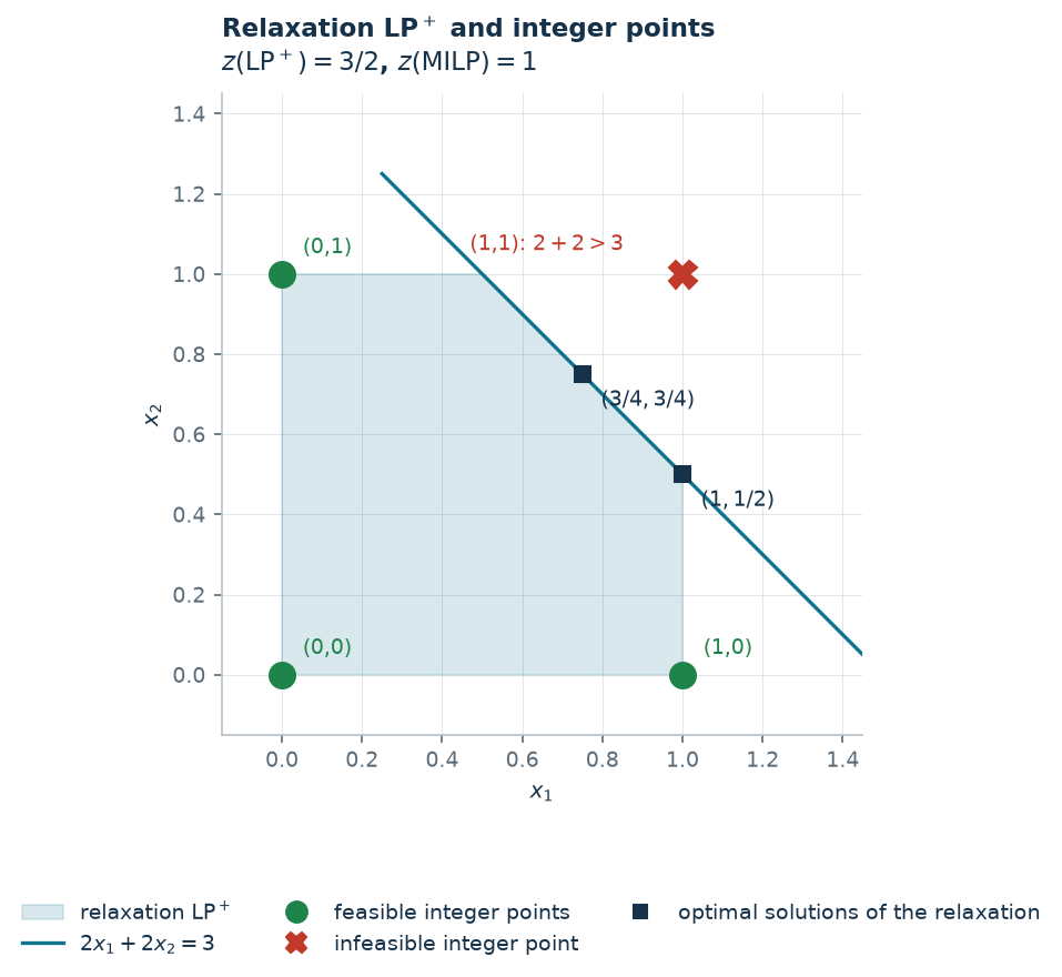
Two distinct lessons: rounding can produce infeasible points, and when it produces feasible ones there is no guarantee on their value; and the difference \(3/2 - 1 = 1/2\) is not the fault of rounding — no feasible integer point is worth more than \(1\).
The two relaxations, and which side they are on
Two versions not to be confused
- relaxation without the bounds \(z(\mathit{LP})\): \(x \in \{0,1\}\) becomes \(x \ge 0\) alone. This is the one whose dual the exercises write by hand.
- relaxation with the bounds \(z(\mathit{LP}^+)\): \(x \in \{0,1\}\)
becomes \(0 \le x \le 1\). This is Gurobi's
relax()and the root relaxation of branch-and-bound.
In a maximisation \(z(\mathit{LP}) \ge z(\mathit{LP}^+) \ge z(\mathit{MILP})\); in a minimisation the directions are reversed. The two coincide when the other constraints already imply \(x \le 1\) — for instance with an assignment constraint \(\sum_m x_{jm} = 1\).
The relaxation removes constraints: every feasible solution of the MILP stays feasible for the relaxation, which therefore optimises over a larger set — and optimising over a larger set cannot give a worse value. In a maximisation the relaxation is an upper bound, in a minimisation a lower bound: in both cases it is an optimistic bound.
Which side each bound comes from
The dual of the relaxation does not give a bound "from the other side". By weak duality, in a minimisation every feasible dual solution is worth at most \(z(\mathit{LP})\), hence at most \(z(\mathit{MILP})\): it sits on the same side as the relaxation. The bound from the other side — the pessimistic one — comes only from a feasible solution of the MILP, that is, from a heuristic or from the solver. Let \((\bar x_1, \bar x_2, \dots, \bar x_n)\) be a feasible solution of the MILP, of value \(\sum_{j=1}^{n} c_j\, \bar x_j\), and \((\bar\pi_1, \bar\pi_2, \dots, \bar\pi_m)\) a feasible solution of the dual of the relaxation, of value \(\sum_{i=1}^{m} b_i\, \bar\pi_i\). In a minimisation the first gives \(\mathit{UB}(\bar x)\) and the second \(\mathit{LB}(\bar\pi)\):
in a maximisation the roles are swapped, the first gives \(\mathit{LB}(\bar x)\) and the second \(\mathit{UB}(\bar\pi)\):
Three "gaps" not to be confused
- Heuristic gap. If \(\bar x\) is the solution built by the heuristic, its value \(\sum_{j=1}^{n} c_j\, \bar x_j\) is the bound \(\mathit{UB}(\bar x)\) in a minimisation (and \(\mathit{LB}(\bar x)\) in a maximisation), and the gap is \(\bigl|\mathit{UB}(\bar x) - z(\mathit{MILP})\bigr| / |z(\mathit{MILP})|\) when the optimum is known — it is the one reported in the exercise tables. When the optimum is not known it is computed against a dual bound, which takes its place.
- Certified gap between two known bounds, without knowing the optimum: \((\mathit{UB} - \mathit{LB})/|\mathit{UB}|\) for a minimisation with \(\mathit{UB} > 0\). It guarantees the optimum lies in the interval, not that it is close to either end.
- The solver's
MIPGap: the same idea, computed by Gurobi from its ownObjValandObjBoundand with its tolerances.
The numerator is always taken in absolute value; if the denominator is zero the relative gap is not written and the absolute difference is reported.
Three patterns that keep coming back
| Name | Constraint | Meaning |
|---|---|---|
| set partitioning | \(\sum_{i \in I} x_i = 1\) | exactly one element of \(I\) |
| set packing | \(\sum_{i \in I} x_i \le 1\) | at most one element of \(I\) |
| set covering | \(\sum_{i \in I} x_i \ge 1\) | at least one element of \(I\) |
A constraint "every job to exactly one machine" is a partitioning; "at most one job per time slot" is a packing; "every zone covered by at least one station" is a covering, which is the direct translation of an OR clause.
What the solver does with the two bounds
A MILP with a bounded feasible set is solved with dedicated algorithms. How they work — how the solution space is explored, how cuts are separated, what to branch on — is not a topic of this course: solution techniques are the subject of a separate course. Only one thing matters here: the two bounds this course teaches how to build by hand are the two sides of the same sandwich the solver tries to close. They are not handed to it: the solver builds its own, with its own heuristics and relaxations.
- The primal bound is a feasible solution, and it gives a value to beat: any part of the space that cannot do better is discarded without being explored.
- The dual bound comes from the relaxation, and says how much one may hope for at most: the closer it is to the integer optimum — that is, the tighter the formulation — the less work is left.
The gap between the two is what the solver reports as MIPGap, and it is also
the only thing one can claim with certainty when the optimum is not reached.
What this chapter has put in your hands
A MIP model is always written with the same five objects: the data, which are known and not decided; the variables, one per decision, with their domain; the objective function, which says what is maximised or minimised; the constraints, one for every sentence of the statement; and the domain of the variables, which is a constraint too, and the easiest to forget.
On a written model one then distinguishes a feasible solution, which satisfies every constraint, and the optimal solution, which among the feasible ones has the best value. Relaxing integrality gives the linear relaxation, an easier problem whose optimum is a bound: pessimistic if it comes from a feasible solution, optimistic if it comes from a relaxation. The distance between the two is the gap.
Code
The complete script — the two relaxations, the rounding
trace and the figure — is
python/cap01_models.py
(reproducible with python3 python/cap01_models.py from the python/ folder).
The same code is available as a notebook —
notebooks/cap01_models.ipynb
— here only to read, though: Python enters the course in
chapter 3, and from that chapter on every page carries its own
Colab badge at the top.
Show the complete script — python/cap01_models.py (116 lines)
"""Chapter 1 -- What is a MIP model: relaxation, rounding, bounds.

Numerical check of the chapter's examples: the rounding counterexample, the two
relaxations (pure and with the bounds kept), the integer optimum and the trace
and the two bounds of the sandwich. Every number quoted in
the notes and on the website comes from here.
"""
import gurobipy as gp
import numpy as np
import pandas as pd
from gurobipy import GRB

from mip import (ammissibile, frazione, nuovo_modello, rilassamento, risolvi,
                 stampa_soluzione, valuta, viola_interezza)
from stile import BLU, CICLO, GRIGIO, ROSSO, TEAL, VERDE, intestazione, plt, salva_dati, salva_figura

R = range

# ---------- 1. THE MODEL OF THE EXAMPLE ----------
intestazione("1. max x1 + x2  s.t.  2x1 + 2x2 <= 3,  x1, x2 binary")


def modello_esempio(binarie=True, superiore=True):
    """Model (1.1) of the chapter.

    binarie=True   -> MILP;  binarie=False -> continuous relaxation
    superiore=True -> the bound x <= 1 is kept (relaxation LP+); False -> only x >= 0
    """
    m = nuovo_modello("rounding")
    tipo = GRB.BINARY if binarie else GRB.CONTINUOUS
    ub = 1.0 if superiore else GRB.INFINITY
    x = m.addVars(2, vtype=tipo, lb=0.0, ub=ub, name="x")
    m.setObjective(x[0] + x[1], GRB.MAXIMIZE)
    m.addConstr(2 * x[0] + 2 * x[1] <= 3, name="resource")
    return m, x


# ---------- 2. THE TWO RELAXATIONS ----------
intestazione("2. The two relaxations: pure (x >= 0) and with the bounds kept (x <= 1)")
m_lp, x_lp = modello_esempio(binarie=False, superiore=False)
zlp = risolvi(m_lp)
print(f"Relaxation without the bounds   z(LP)  = {frazione(zlp)}   solution returned by the solver:")
stampa_soluzione(m_lp)
m_lpp, x_lpp = modello_esempio(binarie=False, superiore=True)
zlpp = risolvi(m_lpp)
vertice = (x_lpp[0].X, x_lpp[1].X)
print(f"Relaxation LP+    z(LP+) = {frazione(zlpp)}   solution returned by the solver: "
      f"({frazione(vertice[0])}, {frazione(vertice[1])})")
print("Both are worth 3/2: the resource constraint already gives x1 + x2 <= 3/2, and")
print("the bound x <= 1 cuts off no point of that segment.")

# every optimal solution of LP+ lies on the segment x1 + x2 = 3/2 inside [0,1]^2
for punto in [(0.75, 0.75), (1.0, 0.5), (0.5, 1.0)]:
    z, viol = valuta(m_lpp, {"x[0]": punto[0], "x[1]": punto[1]})
    assert viol <= 1e-9 and abs(z - 1.5) <= 1e-9
    print(f"  ({frazione(punto[0])}, {frazione(punto[1])}) is feasible for LP+ and is worth "
          f"{frazione(z)}: one of infinitely many optimal solutions.")

# ---------- 3. WHY ROUNDING FAILS ----------
intestazione("3. Rounding the fractional solutions")
m_mip, x_mip = modello_esempio(binarie=True)
for base in [(0.75, 0.75), (1.0, 0.5)]:
    for verso, arr in [("to nearest", lambda v: round(v)), ("downwards", int)]:
        cand = {"x[0]": float(arr(base[0])), "x[1]": float(arr(base[1]))}
        z, viol = valuta(m_mip, cand)
        ok = ammissibile(m_mip, cand)
        print(f"  from ({frazione(base[0])}, {frazione(base[1])}) rounding {verso:11s} -> "
              f"({frazione(cand['x[0]'])}, {frazione(cand['x[1]'])})  "
              f"{'feasible, value ' + frazione(z) if ok else f'INFEASIBLE (violation {viol:g})'}")
assert not ammissibile(m_mip, {"x[0]": 1.0, "x[1]": 1.0})
assert ammissibile(m_mip, {"x[0]": 1.0, "x[1]": 0.0})
# the integrality check really is needed: (1, 1/2) satisfies the linear constraints
assert valuta(m_mip, {"x[0]": 1.0, "x[1]": 0.5})[1] <= 1e-9
assert viola_interezza(m_mip, {"x[0]": 1.0, "x[1]": 0.5}) == 0.5
assert not ammissibile(m_mip, {"x[0]": 1.0, "x[1]": 0.5})
print("  (1, 1/2) satisfies the linear constraints but violates integrality by 1/2:")
print("  continuous feasibility alone does not certify an integer primal bound.")

# ---------- 4. THE INTEGER OPTIMUM ----------
intestazione("4. The integer optimum")
zmilp = risolvi(m_mip)
print(f"z(MILP) = {frazione(zmilp)}   optimal solution:")
stampa_soluzione(m_mip)
print(f"Difference between relaxation and integer optimum: {frazione(zlpp)} - {frazione(zmilp)} = "
      f"{frazione(zlpp - zmilp)}")
salva_dati(pd.DataFrame([{"model": "example 1.1", "z_lp": zlp, "z_lp_rafforzato": zlpp,
                          "z_milp": zmilp}]), "cap01_bound")


# ---------- 6. FIGURE: THE FEASIBLE REGION AND THE INTEGER POINTS ----------
fig, ax = plt.subplots(figsize=(5.4, 5.0))
poligono = [(0, 0), (1, 0), (1, 0.5), (0.5, 1), (0, 1)]
ax.fill(*zip(*poligono), color=TEAL, alpha=0.16, zorder=1, label="relaxation LP$^+$")
ax.plot([0.25, 1.5], [1.25, 0.0], color=TEAL, lw=1.6, zorder=2, label="$2x_1 + 2x_2 = 3$")
for (p, q) in [(0, 0), (1, 0), (0, 1)]:
    ax.plot(p, q, "o", color=VERDE, ms=11, zorder=4)
    ax.annotate(f"({p},{q})", (p, q), textcoords="offset points", xytext=(9, 9),
                fontsize=9, color=VERDE)
ax.plot(1, 1, "X", color=ROSSO, ms=12, zorder=4)
ax.annotate("(1,1): $2+2 > 3$", (1, 1), textcoords="offset points", xytext=(-92, 10),
            fontsize=9, color=ROSSO)
for (p, q), testo in [((0.75, 0.75), "$(3/4,3/4)$"), ((1.0, 0.5), "$(1,1/2)$")]:
    ax.plot(p, q, "s", color=BLU, ms=7, zorder=4)
    ax.annotate(testo, (p, q), textcoords="offset points", xytext=(8, -14), fontsize=9, color=BLU)
ax.plot([], [], "o", color=VERDE, ms=9, label="feasible integer points")
ax.plot([], [], "X", color=ROSSO, ms=9, label="infeasible integer point")
ax.plot([], [], "s", color=BLU, ms=6, label="optimal solutions of the relaxation")
ax.set_xlim(-0.15, 1.45)
ax.set_ylim(-0.15, 1.45)
ax.set_xlabel("$x_1$")
ax.set_ylabel("$x_2$")
ax.set_title("Relaxation LP$^+$ and integer points\n$z(\\mathrm{LP}^+) = 3/2$, $z(\\mathrm{MILP}) = 1$")
ax.legend(loc="upper right", fontsize=8)
ax.set_aspect("equal")
salva_figura(fig, "cap01_rilassamento")
print("Done.")