12.2 An ILP model for the Maximum Clique Problem: the edge formulation¶

Part 2 · Formulations and their properties · Chapter 12 · Chapter 12: Clique problems · Lecture notes, volume 2 (PDF) · Slides · Exercises: Clique problems

The problem of this section is the Maximum Clique Problem (MCP), defined in Chapter 5 «Clique problems», Section 5.2.

Given a simple graph $G=(V,E)$, with $V=\{1,2,\dots,n\}$ and $m$ edges, we denote by

\[ \overline{E} = \big\{\, \{u,v\} : u,v \in V,~ u \neq v,~ \{u,v\} \notin E \,\big\} \]

the set of the non-edges of $G$, that is, the edges of the complement graph $\overline{G}=(V,\overline{E})$.
We introduce the following $n$ binary variables:

\[\begin{equation*} \label{mcpF:var} x_v=\begin{cases}1&\text{if vertex $v$ is selected in the clique}\\[1.5ex]0&\text{otherwise}\end{cases} \qquad\forall v\in V. \tag{12.1} \end{equation*}\]

Using these variables, an Integer Linear Programming (ILP) model for the Maximum Clique Problem (MCP) reads as follows:

\[\begin{align*} && \max \;\; \sum_{v\in V}x_v \label{mcpF:obj} \tag{12.2a}\\[1ex] && \text{subject to} \quad x_u+x_v &\le 1, & \forall\{u,v\}\in\overline{E}, \label{mcpF:nonedge} \tag{12.2b}\\[1ex] && x_v &\in\{0,1\}, & \forall v\in V. \label{mcpF:bin} \tag{12.2c} \end{align*}\]

This ILP model is referred to as the $\mathrm{ILP}_{\mathrm{MCP}}$ model, or edge formulation.

Description of the objective function and constraints of the $\mathrm{ILP}_{\mathrm{MCP}}$ model:
- the linear objective function $\eqref{mcpF:obj}$ maximizes the cardinality of the selected clique;
- constraints $\eqref{mcpF:nonedge}$ ensure that no two non-adjacent vertices are both selected ($|\overline{E}|=\binom{n}{2}-m$ linear constraints, one for each edge of $\overline{G}$);
- finally, constraints $\eqref{mcpF:bin}$ define the variables of the ILP model.
For every non-edge $\{u,v\}$, the constraint $x_u+x_v\le1$ imposes $x_u=1\Rightarrow x_v=0$. The converse is false: $x_u=x_v=0$ is feasible.
Read on $\overline{G}$, the same model is the edge formulation of the MSSP: at most one endpoint of every edge of $\overline{G}$ is selected.

Example 12.1: MCP instance

We consider the graph $G$ with $7$ vertices made of the cycle $1,2,\dots,7,1$ and the chord $\{1,3\}$ (the reference instance of Chapter 5 «Clique problems»), and its complement $\overline{G}$:

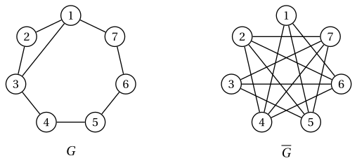
$G$ has $m=8$ edges, and $\overline{G}$ has the $\binom{7}{2}-8=13$ non-edges of $G$:

\[\begin{align*} \overline{E}=\big\{ & \{1,4\},\{1,5\},\{1,6\},\{2,4\},\{2,5\},\{2,6\},\{2,7\},\\ & \{3,5\},\{3,6\},\{3,7\},\{4,6\},\{4,7\},\{5,7\}\big\}. \end{align*}\]

We refer to this MCP instance as Example 12.1.

Example 12.2: $\mathrm{ILP}_{\mathrm{MCP}}$ model

The $\mathrm{ILP}_{\mathrm{MCP}}$ model for the MCP instance of Example 12.1 has $7$ binary variables and one constraint for each of the $13$ edges of $\overline{G}$:

\[ \begin{array}{rrrrrrrrcl} {\max} & {x_1} & {+\,x_2} & {+\,x_3} & {+\,x_4} & {+\,x_5} & {+\,x_6} & {+\,x_7} \\[1ex] \text{subject to} & {x_1} & & & {+\,x_4} & & & & {\le} & {1} \\ & {x_1} & & & & {+\,x_5} & & & {\le} & {1} \\ & {x_1} & & & & & {+\,x_6} & & {\le} & {1} \\ & & {x_2} & & {+\,x_4} & & & & {\le} & {1} \\ & & {x_2} & & & {+\,x_5} & & & {\le} & {1} \\ & & {x_2} & & & & {+\,x_6} & & {\le} & {1} \\ & & {x_2} & & & & & {+\,x_7} & {\le} & {1} \\ & & & {x_3} & & {+\,x_5} & & & {\le} & {1} \\ & & & {x_3} & & & {+\,x_6} & & {\le} & {1} \\ & & & {x_3} & & & & {+\,x_7} & {\le} & {1} \\ & & & & {x_4} & & {+\,x_6} & & {\le} & {1} \\ & & & & {x_4} & & & {+\,x_7} & {\le} & {1} \\ & & & & & {x_5} & & {+\,x_7} & {\le} & {1} \\[1ex] & {x_1}, & {x_2}, & {x_3}, & {x_4}, & {x_5}, & {x_6}, & {x_7} & {\in} & {\{0,1\}} \end{array} \]

An optimal solution $\tilde{\vet x}(\mathrm{ILP}_{\mathrm{MCP}})$ is:

\[ \tilde x_1=\tilde x_2=\tilde x_3=1,~~\tilde x_4=\tilde x_5=\tilde x_6=\tilde x_7=0 \]

The optimal value $z(\mathrm{ILP}_{\mathrm{MCP}})$ is $3=\omega(G)$. The associated optimal solution of the MCP is the clique $\tilde K=\{1,2,3\}$, and it is the unique optimal solution.

12.3 A first Linear Programming relaxation¶

To obtain a Linear Programming (LP) relaxation of the $\mathrm{ILP}_{\mathrm{MCP}}$ model, we relax constraints $\eqref{mcpF:bin}$ into non-negativity constraints. The obtained LP model reads as follows:

\[\begin{align*} && \max \;\; \sum_{v\in V}x_v \label{mcpF:obj-LP0} \tag{12.3a}\\[1ex] && \text{subject to} \quad x_u+x_v &\le 1, & \forall\{u,v\}\in\overline{E}, \label{mcpF:nonedge-LP0} \tag{12.3b}\\[1ex] && x_v &\ge 0, & \forall v\in V. \label{mcpF:nonneg-LP0} \tag{12.3c} \end{align*}\]

This LP model is referred to as the $\mathrm{LP}\text{-}0_{\mathrm{MCP}}$ model.

The upper bounds $x_v\le1$ are not implied in $\mathrm{LP}\text{-}0_{\mathrm{MCP}}$: if a vertex is adjacent to all the others, it belongs to no constraint $\eqref{mcpF:nonedge-LP0}$, and $\mathrm{LP}\text{-}0_{\mathrm{MCP}}$ is unbounded. In Example 12.1 every vertex has a non-edge, and $\mathrm{LP}\text{-}0_{\mathrm{MCP}}$ has an optimal solution.

Example 12.3: $\mathrm{LP}\text{-}0_{\mathrm{MCP}}$ model

The $\mathrm{LP}\text{-}0_{\mathrm{MCP}}$ model for the MCP instance of Example 12.1 is:

\[ \begin{array}{rrrrrrrrcl} {\max} & {x_1} & {+\,x_2} & {+\,x_3} & {+\,x_4} & {+\,x_5} & {+\,x_6} & {+\,x_7} \\[1ex] \text{subject to} & {x_1} & & & {+\,x_4} & & & & {\le} & {1} \\ & {x_1} & & & & {+\,x_5} & & & {\le} & {1} \\ & {x_1} & & & & & {+\,x_6} & & {\le} & {1} \\ & & {x_2} & & {+\,x_4} & & & & {\le} & {1} \\ & & {x_2} & & & {+\,x_5} & & & {\le} & {1} \\ & & {x_2} & & & & {+\,x_6} & & {\le} & {1} \\ & & {x_2} & & & & & {+\,x_7} & {\le} & {1} \\ & & & {x_3} & & {+\,x_5} & & & {\le} & {1} \\ & & & {x_3} & & & {+\,x_6} & & {\le} & {1} \\ & & & {x_3} & & & & {+\,x_7} & {\le} & {1} \\ & & & & {x_4} & & {+\,x_6} & & {\le} & {1} \\ & & & & {x_4} & & & {+\,x_7} & {\le} & {1} \\ & & & & & {x_5} & & {+\,x_7} & {\le} & {1} \\[1ex] & {x_1}, & {x_2}, & {x_3}, & {x_4}, & {x_5}, & {x_6}, & {x_7} & {\ge} & {0} \end{array} \]

An optimal solution $\tilde{\vet x}(\mathrm{LP}\text{-}0_{\mathrm{MCP}})$ is:

\[ \tilde x_1=\tilde x_2=\tilde x_3=\tilde x_4=\tilde x_5=\tilde x_6=\tilde x_7=\frac{1}{2} \]

The optimal value $z(\mathrm{LP}\text{-}0_{\mathrm{MCP}})$ is $\frac{7}{2}$. Accordingly we have the upper bound:

\[ z(\mathrm{ILP}_{\mathrm{MCP}}) \le \frac{7}{2} \]

Using a non-negative dual variable $\pi_{uv}$ for each constraint $\eqref{mcpF:nonedge-LP0}$, the dual model of the $\mathrm{LP}\text{-}0_{\mathrm{MCP}}$ model is:

\[\begin{align*} && \min \;\; \sum_{\{u,v\}\in\overline{E}}\pi_{uv} \label{mcpF:obj-DLP0} \tag{12.4a}\\[1ex] && \text{subject to} \quad \sum_{u:\,\{u,v\}\in\overline{E}}\pi_{uv} &\ge 1, & \forall v\in V, \label{mcpF:cov-DLP0} \tag{12.4b}\\[1ex] && \pi_{uv} &\ge 0, & \forall\{u,v\}\in\overline{E}. \label{mcpF:nonneg-DLP0} \tag{12.4c} \end{align*}\]

This LP model is referred to as the $D(\mathrm{LP}\text{-}0_{\mathrm{MCP}})$ model.

Constraints $\eqref{mcpF:cov-DLP0}$ ask that every vertex is covered by a total weight of at least one on the edges of $\overline{G}$ incident to it: the $D(\mathrm{LP}\text{-}0_{\mathrm{MCP}})$ model is a fractional edge cover of the vertices with the edges of $\overline{G}$.

Example 12.4: $D(\mathrm{LP}\text{-}0_{\mathrm{MCP}})$ model

The dual $D(\mathrm{LP}\text{-}0_{\mathrm{MCP}})$ model for the MCP instance of Example 12.1 has one variable for each edge of $\overline{G}$ and one constraint for each vertex:

\[ \begin{array}{rlcl} {\min} & {\pi_{14}+\pi_{15}+\pi_{16}+\pi_{24}+\pi_{25}+\pi_{26}+\pi_{27}} & & \\ & {+\pi_{35}+\pi_{36}+\pi_{37}+\pi_{46}+\pi_{47}+\pi_{57}} & & \\[1ex] \text{subject to} & {\pi_{14}+\pi_{15}+\pi_{16}} & {\ge} & {1} \\ & {\pi_{24}+\pi_{25}+\pi_{26}+\pi_{27}} & {\ge} & {1} \\ & {\pi_{35}+\pi_{36}+\pi_{37}} & {\ge} & {1} \\ & {\pi_{14}+\pi_{24}+\pi_{46}+\pi_{47}} & {\ge} & {1} \\ & {\pi_{15}+\pi_{25}+\pi_{35}+\pi_{57}} & {\ge} & {1} \\ & {\pi_{16}+\pi_{26}+\pi_{36}+\pi_{46}} & {\ge} & {1} \\ & {\pi_{27}+\pi_{37}+\pi_{47}+\pi_{57}} & {\ge} & {1} \\[1ex] & {\pi_{14},~\pi_{15},~\pi_{16},~\dots,~\pi_{57}} & {\ge} & {0} \end{array} \]

An optimal solution $\tilde{\vet\pi}(D(\mathrm{LP}\text{-}0_{\mathrm{MCP}}))$ gives value $\frac{1}{2}$ to the $7$ edges of the cycle $1,4,7,2,5,3,6,1$ of $\overline{G}$:

\[\begin{align*} &\tilde\pi_{14}=\tilde\pi_{47}=\tilde\pi_{27}=\tilde\pi_{25}=\tilde\pi_{35}=\tilde\pi_{36}=\tilde\pi_{16}=\frac{1}{2},\\ &\tilde\pi_{15}=\tilde\pi_{24}=\tilde\pi_{26}=\tilde\pi_{37}=\tilde\pi_{46}=\tilde\pi_{57}=0 \end{align*}\]

Every vertex lies on two edges of the cycle and receives $\frac{1}{2}+\frac{1}{2}=1$. The optimal value $z(D(\mathrm{LP}\text{-}0_{\mathrm{MCP}}))$ is $\frac{7}{2}$.

12.4 A second Linear Programming relaxation¶

To obtain an LP relaxation of the $\mathrm{ILP}_{\mathrm{MCP}}$ model, we relax constraints $\eqref{mcpF:bin}$ into the bounds $0\le x_v\le 1$. The obtained LP model reads as follows:

\[\begin{align*} && \max \;\; \sum_{v\in V}x_v \label{mcpF:obj-LP} \tag{12.5a}\\[1ex] && \text{subject to} \quad x_u+x_v &\le 1, & \forall\{u,v\}\in\overline{E}, \label{mcpF:nonedge-LP} \tag{12.5b}\\[1ex] && x_v &\le 1, & \forall v\in V, \label{mcpF:ub} \tag{12.5c}\\[1ex] && x_v &\ge 0, & \forall v\in V. \label{mcpF:nonneg-LP} \tag{12.5d} \end{align*}\]

This LP model is referred to as the $\mathrm{LP}_{\mathrm{MCP}}$ model.

Example 12.5: $\mathrm{LP}_{\mathrm{MCP}}$ model

The $\mathrm{LP}_{\mathrm{MCP}}$ model for the MCP instance of Example 12.1 is:

\[ \begin{array}{rrrrrrrrcl} {\max} & {x_1} & {+\,x_2} & {+\,x_3} & {+\,x_4} & {+\,x_5} & {+\,x_6} & {+\,x_7} \\[1ex] \text{subject to} & {x_1} & & & {+\,x_4} & & & & {\le} & {1} \\ & {x_1} & & & & {+\,x_5} & & & {\le} & {1} \\ & {x_1} & & & & & {+\,x_6} & & {\le} & {1} \\ & & {x_2} & & {+\,x_4} & & & & {\le} & {1} \\ & & {x_2} & & & {+\,x_5} & & & {\le} & {1} \\ & & {x_2} & & & & {+\,x_6} & & {\le} & {1} \\ & & {x_2} & & & & & {+\,x_7} & {\le} & {1} \\ & & & {x_3} & & {+\,x_5} & & & {\le} & {1} \\ & & & {x_3} & & & {+\,x_6} & & {\le} & {1} \\ & & & {x_3} & & & & {+\,x_7} & {\le} & {1} \\ & & & & {x_4} & & {+\,x_6} & & {\le} & {1} \\ & & & & {x_4} & & & {+\,x_7} & {\le} & {1} \\ & & & & & {x_5} & & {+\,x_7} & {\le} & {1} \\ & {x_1} & & & & & & & {\le} & {1} \\ & & {x_2} & & & & & & {\le} & {1} \\ & & & {x_3} & & & & & {\le} & {1} \\ & & & & {x_4} & & & & {\le} & {1} \\ & & & & & {x_5} & & & {\le} & {1} \\ & & & & & & {x_6} & & {\le} & {1} \\ & & & & & & & {x_7} & {\le} & {1} \\[1ex] & {x_1}, & {x_2}, & {x_3}, & {x_4}, & {x_5}, & {x_6}, & {x_7} & {\ge} & {0} \end{array} \]

An optimal solution $\tilde{\vet x}(\mathrm{LP}_{\mathrm{MCP}})$ is:

\[ \tilde x_1=\tilde x_2=\tilde x_3=\tilde x_4=\tilde x_5=\tilde x_6=\tilde x_7=\frac{1}{2} \]

The optimal value $z(\mathrm{LP}_{\mathrm{MCP}})$ is $\frac{7}{2}$. Accordingly we have the upper bound:

\[ z(\mathrm{ILP}_{\mathrm{MCP}}) \le \frac{7}{2} \]

Using a non-negative dual variable $\pi_{uv}$ for each constraint $\eqref{mcpF:nonedge-LP}$ and a non-negative dual variable $\lambda_v$ for each constraint $\eqref{mcpF:ub}$, the dual model of the $\mathrm{LP}_{\mathrm{MCP}}$ model is:

\[\begin{align*} && \min \;\; \sum_{\{u,v\}\in\overline{E}}\pi_{uv}+\sum_{v\in V}\lambda_v \label{mcpF:obj-DLP} \tag{12.6a}\\[1ex] && \text{subject to} \quad \sum_{u:\,\{u,v\}\in\overline{E}}\pi_{uv}+\lambda_v &\ge 1, & \forall v\in V, \label{mcpF:cov-DLP} \tag{12.6b}\\[1ex] && \pi_{uv} &\ge 0, & \forall\{u,v\}\in\overline{E}, \label{mcpF:pi-DLP} \tag{12.6c}\\[1ex] && \lambda_v &\ge 0, & \forall v\in V. \label{mcpF:lambda-DLP} \tag{12.6d} \end{align*}\]

This LP model is referred to as the $D(\mathrm{LP}_{\mathrm{MCP}})$ model.

Example 12.6: $D(\mathrm{LP}_{\mathrm{MCP}})$ model

The dual $D(\mathrm{LP}_{\mathrm{MCP}})$ model for the MCP instance of Example 12.1 is:

\[ \begin{array}{rlcl} {\min} & {\pi_{14}+\pi_{15}+\pi_{16}+\pi_{24}+\pi_{25}+\pi_{26}+\pi_{27}} & & \\ & {+\pi_{35}+\pi_{36}+\pi_{37}+\pi_{46}+\pi_{47}+\pi_{57}+\lambda_1} & & \\ & {+\lambda_2+\lambda_3+\lambda_4+\lambda_5+\lambda_6+\lambda_7} & & \\[1ex] \text{subject to} & {\pi_{14}+\pi_{15}+\pi_{16}+\lambda_1} & {\ge} & {1} \\ & {\pi_{24}+\pi_{25}+\pi_{26}+\pi_{27}+\lambda_2} & {\ge} & {1} \\ & {\pi_{35}+\pi_{36}+\pi_{37}+\lambda_3} & {\ge} & {1} \\ & {\pi_{14}+\pi_{24}+\pi_{46}+\pi_{47}+\lambda_4} & {\ge} & {1} \\ & {\pi_{15}+\pi_{25}+\pi_{35}+\pi_{57}+\lambda_5} & {\ge} & {1} \\ & {\pi_{16}+\pi_{26}+\pi_{36}+\pi_{46}+\lambda_6} & {\ge} & {1} \\ & {\pi_{27}+\pi_{37}+\pi_{47}+\pi_{57}+\lambda_7} & {\ge} & {1} \\[1ex] & {\pi_{14},~\pi_{15},~\pi_{16},~\dots,~\pi_{57}} & {\ge} & {0} \\ & {\lambda_1,~\lambda_2,~\lambda_3,~\lambda_4,~\lambda_5,~\lambda_6,~\lambda_7} & {\ge} & {0} \end{array} \]

An optimal solution $(\tilde{\vet\pi},\tilde{\vet\lambda})(D(\mathrm{LP}_{\mathrm{MCP}}))$ is the solution of Example 12.4 with $\tilde\lambda_v=0$ for every $v\in V$:

\[\begin{align*} &\tilde\pi_{14}=\tilde\pi_{47}=\tilde\pi_{27}=\tilde\pi_{25}=\tilde\pi_{35}=\tilde\pi_{36}=\tilde\pi_{16}=\frac{1}{2},\\ &\text{all the other } \tilde\pi_{uv}=0,\qquad \tilde\lambda_1=\tilde\lambda_2=\dots=\tilde\lambda_7=0 \end{align*}\]

The optimal value $z(D(\mathrm{LP}_{\mathrm{MCP}}))$ is $\frac{7}{2}$.

Proposition 12.1: The LP bound can be arbitrarily weak

For every graph $G$ with $n$ vertices, $z(\mathrm{LP}_{\mathrm{MCP}})\ge n/2$. Consequently, the ratio $z(\mathrm{LP}_{\mathrm{MCP}})/z(\mathrm{ILP}_{\mathrm{MCP}})$ is not bounded over all graphs.

Proof

Set $x_v=\frac{1}{2}$ for every vertex. Each constraint $\eqref{mcpF:nonedge-LP}$ becomes $\frac{1}{2}+\frac{1}{2}=1$, and the bounds $\eqref{mcpF:ub}$ and $\eqref{mcpF:nonneg-LP}$ hold, so this is a feasible solution of $\mathrm{LP}_{\mathrm{MCP}}$ of value $n/2$. Graphs without triangles and with an edge have $\omega(G)=2$ for every $n$, and for them the ratio is at least $n/4$. □

The data are integer and the optimal value of the ILP is integer, so $\lfloor z(\mathrm{LP}_{\mathrm{MCP}})\rfloor$ is also a dual bound. On Example 12.1 it gives $\lfloor\frac{7}{2}\rfloor=3=\omega(G)$ by luck; on a graph without triangles it gives $\lfloor n/2\rfloor$, against $\omega(G)=2$.
On the cycle with $5$ vertices $C_5$, where $\omega(C_5)=2$, the point $x_v=\frac{1}{2}$ gives $z(\mathrm{LP}_{\mathrm{MCP}})=\frac{5}{2}$.

12.5 Clique inequalities: a stronger formulation¶

Proposition 12.2: clique inequalities

Let $Q\subseteq V$ be a clique of $\overline{G}$, that is, a stable set of $G$. Then

\[\begin{equation*} \label{mcpF:cliqueineq} \sum_{v\in Q}x_v\le 1 \tag{12.7} \end{equation*}\]

is a valid inequality for $\mathrm{ILP}_{\mathrm{MCP}}$.

Proof

A clique of $G$ and a stable set $Q$ of $G$ share at most one vertex: two common vertices would be both adjacent and non-adjacent. So every feasible solution of $\mathrm{ILP}_{\mathrm{MCP}}$ selects at most one vertex of $Q$. □

Inequalities $\eqref{mcpF:cliqueineq}$ are called clique inequalities, after the clique $Q$ of $\overline{G}$; read on $G$, they are stable set inequalities. The non-edge constraints are the case $|Q|=2$.
If $Q\subseteq Q'$, the inequality of $Q'$ implies the one of $Q$, since all the variables are non-negative. It is enough to write the inequalities of the maximal cliques of $\overline{G}$, whose family we denote by $\mathcal{Q}$.

Using the variables $\eqref{mcpF:var}$, a second ILP model for the Maximum Clique Problem (MCP) reads as follows:

\[\begin{align*} && \max \;\; \sum_{v\in V}x_v \label{mcpF:obj-CL} \tag{12.8a}\\[1ex] && \text{subject to} \quad \sum_{v\in Q}x_v &\le 1, & \forall Q\in\mathcal{Q}, \label{mcpF:cl} \tag{12.8b}\\[1ex] && x_v &\in\{0,1\}, & \forall v\in V. \label{mcpF:bin-CL} \tag{12.8c} \end{align*}\]

This ILP model is referred to as the $\mathrm{ILP}^{\mathrm{CL}}_{\mathrm{MCP}}$ model, or clique formulation.

Description of the objective function and constraints of the $\mathrm{ILP}^{\mathrm{CL}}_{\mathrm{MCP}}$ model:
- the linear objective function $\eqref{mcpF:obj-CL}$ maximizes the cardinality of the selected clique;
- constraints $\eqref{mcpF:cl}$ ensure that at most one vertex of every maximal clique of $\overline{G}$ is selected ($|\mathcal{Q}|$ linear constraints);
- finally, constraints $\eqref{mcpF:bin-CL}$ define the variables of the ILP model.
Every edge of $\overline{G}$ lies in a maximal clique, so each constraint $\eqref{mcpF:nonedge}$ is implied by a constraint $\eqref{mcpF:cl}$: the two models have the same feasible solutions.
The family $\mathcal{Q}$ can be very large: Moon and Moser (1965) showed graphs with $3^{n/3}$ maximal cliques. In practice the inequalities are added only when they are violated, as in Chapter 4 «Valid inequalities» of the module Integer linear programming.

Example 12.7: $\mathrm{ILP}^{\mathrm{CL}}_{\mathrm{MCP}}$ model

The maximal cliques of $\overline{G}$ in Example 12.1 are the $5$ triangles and the $2$ edges

\[ \mathcal{Q}=\big\{\{1,4,6\},\{2,4,6\},\{2,4,7\},\{2,5,7\},\{3,5,7\},\{1,5\},\{3,6\}\big\}, \]

and they give $7$ constraints instead of $13$. The $\mathrm{ILP}^{\mathrm{CL}}_{\mathrm{MCP}}$ model for this MCP instance is:

\[ \begin{array}{rrrrrrrrcl} {\max} & {x_1} & {+\,x_2} & {+\,x_3} & {+\,x_4} & {+\,x_5} & {+\,x_6} & {+\,x_7} \\[1ex] \text{subject to} & {x_1} & & & {+\,x_4} & & {+\,x_6} & & {\le} & {1} \\ & & {x_2} & & {+\,x_4} & & {+\,x_6} & & {\le} & {1} \\ & & {x_2} & & {+\,x_4} & & & {+\,x_7} & {\le} & {1} \\ & & {x_2} & & & {+\,x_5} & & {+\,x_7} & {\le} & {1} \\ & & & {x_3} & & {+\,x_5} & & {+\,x_7} & {\le} & {1} \\ & {x_1} & & & & {+\,x_5} & & & {\le} & {1} \\ & & & {x_3} & & & {+\,x_6} & & {\le} & {1} \\[1ex] & {x_1}, & {x_2}, & {x_3}, & {x_4}, & {x_5}, & {x_6}, & {x_7} & {\in} & {\{0,1\}} \end{array} \]

An optimal solution $\tilde{\vet x}(\mathrm{ILP}^{\mathrm{CL}}_{\mathrm{MCP}})$ is:

\[ \tilde x_1=\tilde x_2=\tilde x_3=1,~~\tilde x_4=\tilde x_5=\tilde x_6=\tilde x_7=0 \]

The optimal value $z(\mathrm{ILP}^{\mathrm{CL}}_{\mathrm{MCP}})$ is $3=\omega(G)$.

To obtain an LP relaxation of the $\mathrm{ILP}^{\mathrm{CL}}_{\mathrm{MCP}}$ model, we relax constraints $\eqref{mcpF:bin-CL}$ into non-negativity constraints. The obtained LP model reads as follows:

\[\begin{align*} && \max \;\; \sum_{v\in V}x_v \label{mcpF:obj-LPCL} \tag{12.9a}\\[1ex] && \text{subject to} \quad \sum_{v\in Q}x_v &\le 1, & \forall Q\in\mathcal{Q}, \label{mcpF:cl-LP} \tag{12.9b}\\[1ex] && x_v &\ge 0, & \forall v\in V. \label{mcpF:nonneg-LPCL} \tag{12.9c} \end{align*}\]

This LP model is referred to as the $\mathrm{LP}^{\mathrm{CL}}_{\mathrm{MCP}}$ model.

Every vertex lies in some maximal clique of $\overline{G}$, so constraints $\eqref{mcpF:cl-LP}$ imply $x_v\le 1$: the bounds $\eqref{mcpF:ub}$ are not needed.
Each constraint $\eqref{mcpF:nonedge-LP}$ is implied by a constraint $\eqref{mcpF:cl-LP}$. Hence the feasible region of $\mathrm{LP}^{\mathrm{CL}}_{\mathrm{MCP}}$ is contained in that of $\mathrm{LP}_{\mathrm{MCP}}$, and

\[ \omega(G) \;\le\; z(\mathrm{LP}^{\mathrm{CL}}_{\mathrm{MCP}}) \;\le\; z(\mathrm{LP}_{\mathrm{MCP}}). \]

Example 12.8: $\mathrm{LP}^{\mathrm{CL}}_{\mathrm{MCP}}$ model

The $\mathrm{LP}^{\mathrm{CL}}_{\mathrm{MCP}}$ model for the MCP instance of Example 12.1 is:

\[ \begin{array}{rrrrrrrrcl} {\max} & {x_1} & {+\,x_2} & {+\,x_3} & {+\,x_4} & {+\,x_5} & {+\,x_6} & {+\,x_7} \\[1ex] \text{subject to} & {x_1} & & & {+\,x_4} & & {+\,x_6} & & {\le} & {1} \\ & & {x_2} & & {+\,x_4} & & {+\,x_6} & & {\le} & {1} \\ & & {x_2} & & {+\,x_4} & & & {+\,x_7} & {\le} & {1} \\ & & {x_2} & & & {+\,x_5} & & {+\,x_7} & {\le} & {1} \\ & & & {x_3} & & {+\,x_5} & & {+\,x_7} & {\le} & {1} \\ & {x_1} & & & & {+\,x_5} & & & {\le} & {1} \\ & & & {x_3} & & & {+\,x_6} & & {\le} & {1} \\[1ex] & {x_1}, & {x_2}, & {x_3}, & {x_4}, & {x_5}, & {x_6}, & {x_7} & {\ge} & {0} \end{array} \]

The point $\bar x_v=\frac{1}{2}$ is no longer feasible: $\bar x_1+\bar x_4+\bar x_6=\frac{3}{2}>1$. Summing the three constraints of $\{1,4,6\}$, $\{2,5,7\}$ and $\{3,5,7\}$ gives

\[ \sum_{v=1}^{7}x_v + x_5 + x_7 \le 3 \quad\Longrightarrow\quad \sum_{v=1}^{7}x_v\le 3. \]

An optimal solution $\tilde{\vet x}(\mathrm{LP}^{\mathrm{CL}}_{\mathrm{MCP}})$ is:

\[ \tilde x_1=\tilde x_2=\tilde x_3=1,~~\tilde x_4=\tilde x_5=\tilde x_6=\tilde x_7=0 \]

The optimal value $z(\mathrm{LP}^{\mathrm{CL}}_{\mathrm{MCP}})$ is $3=\omega(G)$: the LP bound drops from $\frac{7}{2}$ to $3$ and closes the gap.

Clique inequalities do not always close the gap. On $C_5$ the complement is again a cycle with $5$ vertices, whose maximal cliques are its edges: the two formulations coincide and $z(\mathrm{LP}^{\mathrm{CL}}_{\mathrm{MCP}})= \frac{5}{2}>2=\omega(C_5)$.
If $C$ is a cycle of $\overline{G}$ with an odd number of vertices and no chord, then $\sum_{v\in C}x_v\le(|C|-1)/2$ is a valid inequality (an odd cycle inequality): a stable set of $\overline{G}$ takes at most $(|C|-1)/2$ vertices of $C$. For $C_5$ it reads $x_1+\dots+x_5\le 2$ and closes the gap.

12.6 The relation with vertex coloring¶

In a coloring of $G$ the vertices of a clique take pairwise different colors, hence (Chapter 4 «Coloring problems»)

\[ \omega(G)\le\chi(G). \]

Here we place the LP bound of the clique formulation between the two numbers.
The maximal cliques of $\overline{G}$ are the maximal stable sets of $G$, and a color class is a stable set. We introduce the following $|\mathcal{Q}|$ binary variables:

\[\begin{equation*} \label{mcpF:var-col} y_Q=\begin{cases}1&\text{if the stable set $Q$ is a color class}\\[1.5ex]0&\text{otherwise}\end{cases} \qquad\forall Q\in\mathcal{Q}. \tag{12.10} \end{equation*}\]

Using these variables, an ILP model for the Vertex Coloring Problem (VCP) reads as follows:

\[\begin{align*} && \min \;\; \sum_{Q\in\mathcal{Q}}y_Q \label{mcpF:obj-col} \tag{12.11a}\\[1ex] && \text{subject to} \quad \sum_{Q\in\mathcal{Q}:\,v\in Q}y_Q &\ge 1, & \forall v\in V, \label{mcpF:cov-col} \tag{12.11b}\\[1ex] && y_Q &\in\{0,1\}, & \forall Q\in\mathcal{Q}. \label{mcpF:bin-col} \tag{12.11c} \end{align*}\]

This ILP model is referred to as the $\mathrm{ILP}^{\mathrm{ST}}_{\mathrm{VCP}}$ model, or stable set formulation of the VCP.

Description of the objective function and constraints of the $\mathrm{ILP}^{\mathrm{ST}}_{\mathrm{VCP}}$ model:
- the linear objective function $\eqref{mcpF:obj-col}$ minimizes the number of color classes;
- constraints $\eqref{mcpF:cov-col}$ ensure that every vertex belongs to at least one chosen stable set ($n$ linear constraints);
- finally, constraints $\eqref{mcpF:bin-col}$ define the variables of the ILP model.
Its optimal value is $\chi(G)$: a vertex covered by two chosen sets is kept in one of them, and every subset of a stable set is stable, so the chosen sets give a coloring with the same number of colors.

Using a non-negative dual variable $\pi_Q$ for each constraint $\eqref{mcpF:cl-LP}$, the dual model of the $\mathrm{LP}^{\mathrm{CL}}_{\mathrm{MCP}}$ model is:

\[\begin{align*} && \min \;\; \sum_{Q\in\mathcal{Q}}\pi_Q \label{mcpF:obj-DLPCL} \tag{12.12a}\\[1ex] && \text{subject to} \quad \sum_{Q\in\mathcal{Q}:\,v\in Q}\pi_Q &\ge 1, & \forall v\in V, \label{mcpF:cov-DLPCL} \tag{12.12b}\\[1ex] && \pi_Q &\ge 0, & \forall Q\in\mathcal{Q}. \label{mcpF:nonneg-DLPCL} \tag{12.12c} \end{align*}\]

This LP model is referred to as the $D(\mathrm{LP}^{\mathrm{CL}}_{\mathrm{MCP}})$ model.

Proposition 12.3: clique bound from LP duality

The dual $D(\mathrm{LP}^{\mathrm{CL}}_{\mathrm{MCP}})$ model is the LP relaxation of the $\mathrm{ILP}^{\mathrm{ST}}_{\mathrm{VCP}}$ model, with the variables $\pi_Q$ in place of $y_Q$. Hence

\[ \omega(G)\;\le\; z(\mathrm{LP}^{\mathrm{CL}}_{\mathrm{MCP}}) \;\le\; \chi(G). \]

Proof

Relaxing constraints $\eqref{mcpF:bin-col}$ into $y_Q\ge 0$ gives exactly the model (12.12), with $y_Q$ in place of $\pi_Q$. By strong duality $z(\mathrm{LP}^{\mathrm{CL}}_{\mathrm{MCP}})=z(D(\mathrm{LP}^{\mathrm{CL}}_{\mathrm{MCP}}))$. The first inequality holds because $\mathrm{LP}^{\mathrm{CL}}_{\mathrm{MCP}}$ is a relaxation of the MCP. The second one holds because $D(\mathrm{LP}^{\mathrm{CL}}_{\mathrm{MCP}})$ is a relaxation of the $\mathrm{ILP}^{\mathrm{ST}}_{\mathrm{VCP}}$ model, a minimization problem with optimal value $\chi(G)$. □

The common value $z(\mathrm{LP}^{\mathrm{CL}}_{\mathrm{MCP}})$ is called the fractional chromatic number of $G$. The clique formulation of the MCP and the stable set formulation of the VCP are two faces of the same LP.

Example 12.9: $D(\mathrm{LP}^{\mathrm{CL}}_{\mathrm{MCP}})$ model

The dual $D(\mathrm{LP}^{\mathrm{CL}}_{\mathrm{MCP}})$ model for the MCP instance of Example 12.1 has one variable for each maximal stable set of $G$ ($\pi_{146}$ for $Q=\{1,4,6\}$, and so on):

\[ \begin{array}{rrrrrrrrcl} {\min} & {\pi_{146}} & {+\,\pi_{246}} & {+\,\pi_{247}} & {+\,\pi_{257}} & {+\,\pi_{357}} & {+\,\pi_{15}} & {+\,\pi_{36}} \\[1ex] \text{subject to} & {\pi_{146}} & & & & & {+\,\pi_{15}} & & {\ge} & {1} \\ & & {\pi_{246}} & {+\,\pi_{247}} & {+\,\pi_{257}} & & & & {\ge} & {1} \\ & & & & & {\pi_{357}} & & {+\,\pi_{36}} & {\ge} & {1} \\ & {\pi_{146}} & {+\,\pi_{246}} & {+\,\pi_{247}} & & & & & {\ge} & {1} \\ & & & & {\pi_{257}} & {+\,\pi_{357}} & {+\,\pi_{15}} & & {\ge} & {1} \\ & {\pi_{146}} & {+\,\pi_{246}} & & & & & {+\,\pi_{36}} & {\ge} & {1} \\ & & & {\pi_{247}} & {+\,\pi_{257}} & {+\,\pi_{357}} & & & {\ge} & {1} \\[1ex] & {\pi_{146}}, & {\pi_{246}}, & {\pi_{247}}, & {\pi_{257}}, & {\pi_{357}}, & {\pi_{15}}, & {\pi_{36}} & {\ge} & {0} \end{array} \]

An optimal solution $\tilde{\vet\pi}(D(\mathrm{LP}^{\mathrm{CL}}_{\mathrm{MCP}}))$ gives value $1$ to the multipliers used in Example 12.8:

\[ \tilde\pi_{146}=\tilde\pi_{257}=\tilde\pi_{357}=1,~~\tilde\pi_{246}=\tilde\pi_{247}=\tilde\pi_{15}=\tilde\pi_{36}=0 \]

The optimal value $z(D(\mathrm{LP}^{\mathrm{CL}}_{\mathrm{MCP}}))$ is $3$.

Example 12.10: the chain $\omega\le z(\mathrm{LP}^{\mathrm{CL}}_{\mathrm{MCP}})\le\chi$

On Example 12.1, the $\mathrm{ILP}^{\mathrm{ST}}_{\mathrm{VCP}}$ model is:

\[ \begin{array}{rrrrrrrrcl} {\min} & {y_{146}} & {+\,y_{246}} & {+\,y_{247}} & {+\,y_{257}} & {+\,y_{357}} & {+\,y_{15}} & {+\,y_{36}} \\[1ex] \text{subject to} & {y_{146}} & & & & & {+\,y_{15}} & & {\ge} & {1} \\ & & {y_{246}} & {+\,y_{247}} & {+\,y_{257}} & & & & {\ge} & {1} \\ & & & & & {y_{357}} & & {+\,y_{36}} & {\ge} & {1} \\ & {y_{146}} & {+\,y_{246}} & {+\,y_{247}} & & & & & {\ge} & {1} \\ & & & & {y_{257}} & {+\,y_{357}} & {+\,y_{15}} & & {\ge} & {1} \\ & {y_{146}} & {+\,y_{246}} & & & & & {+\,y_{36}} & {\ge} & {1} \\ & & & {y_{247}} & {+\,y_{257}} & {+\,y_{357}} & & & {\ge} & {1} \\[1ex] & {y_{146}}, & {y_{246}}, & {y_{247}}, & {y_{257}}, & {y_{357}}, & {y_{15}}, & {y_{36}} & {\in} & {\{0,1\}} \end{array} \]

The integer point $\tilde y_{146}=\tilde y_{257}=\tilde y_{357}=1$, all the other variables equal to $0$, is the solution of Example 12.9: it is a coloring with $3$ colors, the classes $\{1,4,6\}$, $\{2,5,7\}$ and $\{3\}$. Hence $\chi(G)=3$, and the chain reads $3\le 3\le 3$.
On $C_5$, with vertices $1,\dots,5$, the maximal stable sets are the $5$ non-edges. Setting $\pi_Q=\frac{1}{2}$ on each of them gives every vertex a total of $1$, so the dual has value $\frac{5}{2}$, as the primal. The chain reads

\[ \omega(C_5)=2 \;<\; z(\mathrm{LP}^{\mathrm{CL}}_{\mathrm{MCP}})=\frac{5}{2} \;<\; \chi(C_5)=3 . \]

12.7 Stable sets on the complement graph¶

The problem of this section is the Maximum Stable Set Problem (MSSP), defined in Chapter 5 «Clique problems», Section 5.2.

Given a simple graph $G=(V,E)$, with $V=\{1,2,\dots,n\}$ and $m$ edges, we introduce the following $n$ binary variables:

\[\begin{equation*} \label{mcpF:var-mssp} x_v=\begin{cases}1&\text{if vertex $v$ is selected in the stable set}\\[1.5ex]0&\text{otherwise}\end{cases} \qquad\forall v\in V. \tag{12.13} \end{equation*}\]

Using these variables, an Integer Linear Programming (ILP) model for the Maximum Stable Set Problem (MSSP) reads as follows:

\[\begin{align*} && \max \;\; \sum_{v\in V}x_v \label{mcpF:obj-mssp} \tag{12.14a}\\[1ex] && \text{subject to} \quad x_u+x_v &\le 1, & \forall\{u,v\}\in E, \label{mcpF:edge-mssp} \tag{12.14b}\\[1ex] && x_v &\in\{0,1\}, & \forall v\in V. \label{mcpF:bin-mssp} \tag{12.14c} \end{align*}\]

This ILP model is referred to as the $\mathrm{ILP}_{\mathrm{MSSP}}$ model, or edge formulation of the MSSP.

Description of the objective function and constraints of the $\mathrm{ILP}_{\mathrm{MSSP}}$ model:
- the linear objective function $\eqref{mcpF:obj-mssp}$ maximizes the cardinality of the selected stable set;
- constraints $\eqref{mcpF:edge-mssp}$ ensure that no two adjacent vertices are both selected ($m$ linear constraints, one for each edge of $G$);
- finally, constraints $\eqref{mcpF:bin-mssp}$ define the variables of the ILP model.
The $\mathrm{ILP}_{\mathrm{MSSP}}$ model on $G$ is the $\mathrm{ILP}_{\mathrm{MCP}}$ model on $\overline{G}$: the non-edges of $\overline{G}$ are the edges of $G$. This is the identity $\alpha(G)=\omega(\overline{G})$ written as a model.

Example 12.11: $\mathrm{ILP}_{\mathrm{MSSP}}$ model

We consider the graph $G$ of Example 12.1, the cycle $1,2,\dots,7,1$ with the chord $\{1,3\}$, and we look for a maximum stable set of $G$. The $\mathrm{ILP}_{\mathrm{MSSP}}$ model has $7$ binary variables and one constraint for each of the $8$ edges of $G$:

\[ \begin{array}{rrrrrrrrcl} {\max} & {x_1} & {+\,x_2} & {+\,x_3} & {+\,x_4} & {+\,x_5} & {+\,x_6} & {+\,x_7} \\[1ex] \text{subject to} & {x_1} & {+\,x_2} & & & & & & {\le} & {1} \\ & {x_1} & & {+\,x_3} & & & & & {\le} & {1} \\ & {x_1} & & & & & & {+\,x_7} & {\le} & {1} \\ & & {x_2} & {+\,x_3} & & & & & {\le} & {1} \\ & & & {x_3} & {+\,x_4} & & & & {\le} & {1} \\ & & & & {x_4} & {+\,x_5} & & & {\le} & {1} \\ & & & & & {x_5} & {+\,x_6} & & {\le} & {1} \\ & & & & & & {x_6} & {+\,x_7} & {\le} & {1} \\[1ex] & {x_1}, & {x_2}, & {x_3}, & {x_4}, & {x_5}, & {x_6}, & {x_7} & {\in} & {\{0,1\}} \end{array} \]

An optimal solution $\tilde{\vet x}(\mathrm{ILP}_{\mathrm{MSSP}})$ is:

\[ \tilde x_1=\tilde x_4=\tilde x_6=1,~~\tilde x_2=\tilde x_3=\tilde x_5=\tilde x_7=0 \]

The optimal value $z(\mathrm{ILP}_{\mathrm{MSSP}})$ is $3=\alpha(G)$. The optimal solution is not unique: the maximum stable sets of $G$ are $\{1,4,6\}$, $\{2,4,6\}$, $\{2,4,7\}$, $\{2,5,7\}$ and $\{3,5,7\}$, the five triangles of $\overline{G}$.

A stable set and a clique of $G$ share at most one vertex, so for every clique $K$ of $G$ the clique inequality $\sum_{v\in K}x_v\le 1$ is valid, and it implies the constraints $\eqref{mcpF:edge-mssp}$ of the edges of $K$. As for the MCP, it is enough to write the inequalities of the family $\mathcal{K}$ of the maximal cliques of $G$.

Using the variables $\eqref{mcpF:var-mssp}$, a second ILP model for the Maximum Stable Set Problem (MSSP) reads as follows:

\[\begin{align*} && \max \;\; \sum_{v\in V}x_v \label{mcpF:obj-mssp-cl} \tag{12.15a}\\[1ex] && \text{subject to} \quad \sum_{v\in K}x_v &\le 1, & \forall K\in\mathcal{K}, \label{mcpF:cl-mssp} \tag{12.15b}\\[1ex] && x_v &\in\{0,1\}, & \forall v\in V. \label{mcpF:bin-mssp-cl} \tag{12.15c} \end{align*}\]

This ILP model is referred to as the $\mathrm{ILP}^{\mathrm{CL}}_{\mathrm{MSSP}}$ model, or clique formulation of the MSSP.

Description of the objective function and constraints of the $\mathrm{ILP}^{\mathrm{CL}}_{\mathrm{MSSP}}$ model:
- the linear objective function $\eqref{mcpF:obj-mssp-cl}$ maximizes the cardinality of the selected stable set;
- constraints $\eqref{mcpF:cl-mssp}$ ensure that at most one vertex of every maximal clique of $G$ is selected ($|\mathcal{K}|$ linear constraints);
- finally, constraints $\eqref{mcpF:bin-mssp-cl}$ define the variables of the ILP model.
The $\mathrm{ILP}^{\mathrm{CL}}_{\mathrm{MSSP}}$ model on $G$ is the $\mathrm{ILP}^{\mathrm{CL}}_{\mathrm{MCP}}$ model on $\overline{G}$, and its LP relaxation is at least as strong as that of the $\mathrm{ILP}_{\mathrm{MSSP}}$ model.

Example 12.12: $\mathrm{ILP}^{\mathrm{CL}}_{\mathrm{MSSP}}$ model

The maximal cliques of the graph $G$ of Example 12.1 are the triangle $\{1,2,3\}$ and the five edges $\{3,4\},\{4,5\},\{5,6\},\{6,7\},\{1,7\}$. The $\mathrm{ILP}^{\mathrm{CL}}_{\mathrm{MSSP}}$ model replaces the three constraints of the triangle with one constraint, and has $6$ constraints:

\[ \begin{array}{rrrrrrrrcl} {\max} & {x_1} & {+\,x_2} & {+\,x_3} & {+\,x_4} & {+\,x_5} & {+\,x_6} & {+\,x_7} \\[1ex] \text{subject to} & {x_1} & {+\,x_2} & {+\,x_3} & & & & & {\le} & {1} \\ & & & {x_3} & {+\,x_4} & & & & {\le} & {1} \\ & & & & {x_4} & {+\,x_5} & & & {\le} & {1} \\ & & & & & {x_5} & {+\,x_6} & & {\le} & {1} \\ & & & & & & {x_6} & {+\,x_7} & {\le} & {1} \\ & {x_1} & & & & & & {+\,x_7} & {\le} & {1} \\[1ex] & {x_1}, & {x_2}, & {x_3}, & {x_4}, & {x_5}, & {x_6}, & {x_7} & {\in} & {\{0,1\}} \end{array} \]

The optimal solution $\tilde x_1=\tilde x_4=\tilde x_6=1$ of Example 12.11 is optimal here too, with value $z(\mathrm{ILP}^{\mathrm{CL}}_{\mathrm{MSSP}})=3$. The LP relaxations differ (Gurobi): the edge formulation, with $0\le x_v\le 1$, has optimal value $\frac{7}{2}$ at $x_v=\frac{1}{2}$, while the clique formulation has optimal value $3$, attained by $x_2=x_5=x_7=1$.

Next: 12.8 ILP models for the weighted variants