Vertex coloring: the DSATUR branch-and-bound

Part 6 · Ad hoc algorithms · Chapter 42 · Lecture notes, volume 6 (PDF) · Slides · Exercises: Vertex coloring (VCP) · App: Vertex coloring: the DSATUR branch-and-bound

Prerequisites

• From the module Integer linear programming, Chapter 7 «Branch-and-bound»: branching and bounding operations, the problem list, the pruning criteria, the bounds \(\LB\) and \(\UB\).

• From this module, Chapter 4 «Coloring problems»: the vertex coloring problem, cliques, stable sets and the clique bound \(\omega(G)\le\chi(G)\).

• From this module, Chapter 30 «Constructive heuristics»: the saturation degree and the \(DSATUR\) heuristic.

Objectives

At the end of this chapter you will be able to:

• describe a node of the tree as a partial coloring, with its colors used and its saturation degrees;

• branch on the vertex of maximum saturation degree, with one child per feasible color and one new color;

• compute the upper bound with \(DSATUR\), the lower bound with a greedy clique, and prune a node;

• execute the DSATUR branch-and-bound algorithm by hand and prove that it is exact.

The problem of this chapter is the vertex coloring problem (VCP): its definition and its assumptions are on its page. On a graph \(G=(V,E)\), its optimal value is the chromatic number \(\chi(G)\).

42.1 The algorithm for the VCP

Definition 42.1: branching node and partial coloring

In the DSATUR branch-and-bound algorithm, the colors are the integers \(1,2,3,\dots\), and a branching node \(k\) of the tree is a partial coloring:

1. a subset of colored vertices \(\rightsquigarrow\) denoted \(V^k \subseteq V\);

2. a color \(\mathit{col}^k(v)\) for every \(v \in V^k\), with \(\mathit{col}^k(u)\neq\mathit{col}^k(v)\) for all \(\{u,v\}\in E\), \(u,v\in V^k\);

3. a subset of uncolored vertices \(\rightsquigarrow\) denoted \(U^k := V \setminus V^k\).

The colors used at node \(k\) are \(1,2,\dots,q(k)\), where \(q(k)\) is the number of colors used, and the color classes are \(Q^k_c := \{\, v\in V^k : \mathit{col}^k(v)=c \,\}\), \(c=1,\dots,q(k)\). For an uncolored vertex \(v \in U^k\):

\[\begin{align*} \mathit{sat}_k(v) &:= \big|\{\, \mathit{col}^k(u) : u \in N(v)\cap V^k \,\}\big| && \text{(\textbf{saturation degree})},\\[1ex] \mathit{du}_k(v) &:= |N(v)\cap U^k| && \text{(degree among the uncolored vertices)},\\[1ex] F_k(v) &:= \{\, c\in\{1,\dots,q(k)\} : Q^k_c\cap N(v)=\emptyset \,\} && \text{(\textbf{feasible colors})}. \end{align*}\]

• The saturation degree counts the different colors among the colored neighbours of \(v\), and \(|F_k(v)| = q(k)-\mathit{sat}_k(v)\).

• A node with \(U^k=\emptyset\) is a complete coloring: a feasible solution of the VCP with \(q(k)\) colors.

A node of the tree is a partial coloring; each child colors one more vertex. No LP problem is solved: the bounds of a node come from counting colors.

42.1.1 Branching

• Branching vertex. At node \(k\) we branch on the uncolored vertex \(v\) of maximum saturation degree \(\mathit{sat}_k(v)\); ties are broken by the largest \(\mathit{du}_k(v)\), and then by the smallest index. This is the rule of the \(DSATUR\) heuristic (Brélaz, 1979).

• Children. The children of node \(k\) give a color to \(v\):

  1. one child for every feasible color \(c\in F_k(v)\), in increasing order of \(c\);

  2. one child with the new color \(q(k)+1\).

• The colors \(q(k)+2, q(k)+3,\dots\) are not used: a child with color \(q(k)+2\) would differ from the child with color \(q(k)+1\) only by the name of an empty color. The children are no symmetric copies of each other.

• The most saturated vertex has the fewest children: \(|F_k(v)|+1\). If \(F_k(v)=\emptyset\), the node has only the child with the new color.

The branching vertex is the most constrained one; its children are its feasible colors plus one new color, so two children never describe the same coloring with the colors renamed.

42.1.2 Bounds and pruning

• The VCP is a minimization problem: the incumbent solution gives the upper bound \(\UB\), and a lower bound comes from a clique.

• Upper bound. Before branching, the \(DSATUR\) heuristic of Chapter 30 «Constructive heuristics» gives the first incumbent solution, and \(\UB\) is its number of colors.

• Greedy clique. The vertices are scanned by non-increasing degree (ties: smallest index), and a vertex enters \(K\) if it is adjacent to all the vertices already in \(K\). The set \(K=\{k_1,\dots,k_r\}\) is a maximal clique, and \(\LB := r \le \omega(G)\le\chi(G)\).

• Pre-coloring. The vertices of \(K\) need \(r\) different colors in every coloring, and the names of the colors are arbitrary: the root node colors \(k_i\) with color \(i\), \(i=1,\dots,r\). This breaks the symmetry of the first \(r\) colors.

• Lower bound of a node. The colors of a node are never removed in its subtree, so every complete coloring below node \(k\) uses at least \(q(k)\) colors:

  \[ \LB(k) \;:=\; \max\{\, q(k),\; |K| \,\} \;=\; q(k), \]

  where the equality holds because the clique is pre-colored.

• Pruning. The number of colors is an integer, so a node can lead to a better solution only if it uses fewer than \(\UB\) colors. Node \(k\) is pruned by bound if

  \[ q(k) \;\ge\; \UB . \]

• Complete coloring. A node with \(U^k=\emptyset\) and \(q(k)<\UB\) is a new incumbent solution: \(\UB \leftarrow q(k)\), and the nodes of the list with \(q \ge \UB\) are removed. If \(\UB=|K|\), the incumbent solution is optimal and the algorithm stops.

\(DSATUR\) gives \(\UB\), a greedy clique gives \(\LB\); a node is pruned as soon as it uses \(\UB\) colors, because its subtree cannot contain a coloring with fewer colors.

42.1.3 Node selection and pseudocode

• The tree is explored depth first: the list \(L\) is a stack, the children of a node are evaluated in increasing order of color, and the child with the smallest color is extracted first.

• The nodes are numbered in the order of evaluation. A child is evaluated as soon as it is created: the evaluation only computes \(q\) and checks whether the coloring is complete.

Algorithm

• Input: a VCP instance, i.e., a graph \(G=(V,E)\).

• Output: an optimal coloring and the chromatic number \(\chi(G)\).

• Step 0: Initialization

  1. Run \(DSATUR\): set the incumbent solution to its coloring and \(\UB\) to its number of colors.

  2. Find the greedy clique \(K=\{k_1,\dots,k_r\}\) and set \(\LB \leftarrow r\). If \(\LB=\UB\), the incumbent solution is optimal. STOP.

  3. Create node \(1\) with \(\mathit{col}^1(k_i)=i\), \(i=1,\dots,r\), and \(q(1)=r\). Insert node \(1\) into the list \(L\) and set the node counter \(c\leftarrow 1\).

• Step 1: Optimality check

  If \(L\) is empty, \(\UB\) is the optimal value and the incumbent solution is optimal. STOP.

• Step 2: Branching-node selection

  Remove from \(L\) the node \(k\) inserted last.

• Step 3: Branching

  Select \(v\in U^k\) of maximum \(\mathit{sat}_k(v)\), then maximum \(\mathit{du}_k(v)\), then smallest index. For each color \(a\in F_k(v)\cup\{q(k)+1\}\), in increasing order, create node \(c+1\) as node \(k\) with \(\mathit{col}(v)=a\), evaluate it with the node sub-procedure, and set \(c\leftarrow c+1\). Insert the surviving children into \(L\) in decreasing order of color and go to Step 1.

• In Step 3, the counter \(c\) of the nodes gives the next free index, and \(a\) is the color given to \(v\) in the child.

• This is the pseudocode of the node sub-procedure.

Algorithm

• Input: a node \(h\), i.e., a partial coloring with \(q(h)\) colors.

• Step 1: Bounding operations

  1. If \(q(h)\ge\UB\), the node is pruned by bound. STOP.

  2. If \(U^h=\emptyset\), update the upper bound and the incumbent solution: \(\UB\leftarrow q(h)\). Remove from \(L\) all the nodes with \(q\ge\UB\). If \(\UB=\LB\), the incumbent solution is optimal: STOP the algorithm. Otherwise STOP.

• Step 2: Survival

  The node survives: it is inserted into \(L\) in Step 3. STOP.

42.1.4 Correctness

Proposition 42.2: no-symmetry branching

Consider the tree of the DSATUR branch-and-bound algorithm without pruning. Its leaves are complete colorings, and every partition of \(V\) into stable sets, i.e., every feasible solution of the VCP, is the set of color classes of exactly one leaf.

Proof

Let \(\mathcal{Q}\) be a partition of \(V\) into stable sets. The vertices of the clique \(K\) are pairwise adjacent, so they lie in \(r\) different classes; we give the name \(i\) to the class of \(k_i\).

1. Existence. We follow a path from the root and keep this invariant: the classes of the node are the classes of \(\mathcal{Q}\) restricted to \(V^k\), each with its name. The root satisfies it. At node \(k\), let \(v\) be the branching vertex and \(Q\in\mathcal{Q}\) its class.

   • If \(Q\) already has a colored vertex, with name \(c\), then no neighbour of \(v\) has color \(c\), because \(Q\) is stable. Hence \(c\in F_k(v)\), and the child with color \(c\) keeps the invariant.

   • Otherwise \(Q\) has no colored vertex yet: the child with the new color \(q(k)+1\) keeps the invariant, and \(Q\) gets the name \(q(k)+1\).

   Every step colors one vertex, so after \(|U^1|\) steps we reach a leaf whose classes are \(\mathcal{Q}\).

2. Uniqueness. Two different children of a node put \(v\) in different classes: with the colored vertices of two different colors, or with one of them and alone. The partition restricted to \(V^k\cup\{v\}\) differs, so the leaves below two different children give different partitions. □

• The algorithm is exact. A node is pruned only if \(q(k)\ge\UB\), and every leaf below it uses at least \(q(k)\) colors: no coloring with fewer than \(\UB\) colors is lost. When the list is empty, \(\UB=\chi(G)\).

• Without the new-color rule, every partition with \(q\) classes would appear once for every way of naming its classes with the colors \(1,\dots,\UB-1\): the tree would contain many symmetric copies of the same solution.

Without pruning, the tree enumerates every feasible solution of the VCP exactly once, up to a renaming of the colors. The pruning by bound removes only subtrees with at least \(\UB\) colors: the algorithm is exact.

42.2 A worked example

Example 42.1: DSATUR branch-and-bound on the Petersen graph

We consider the Petersen graph, the reference instance of Chapter 4 «Coloring problems», with \(n=10\) vertices, \(m=15\) edges and all degrees equal to \(3\):

\[ \begin{aligned} E = \big\{~ & \{1,2\},~ \{1,5\},~ \{1,6\},~ \{2,3\},~ \{2,7\},~ \{3,4\},~ \{3,8\},~ \{4,5\},\\ & \{4,9\},~ \{5,10\},~ \{6,8\},~ \{6,9\},~ \{7,9\},~ \{7,10\},~ \{8,10\} ~\big\}. \end{aligned} \]

The DSATUR branch-and-bound algorithm uses the rules of Section 42.1: branching on the most saturated vertex, depth-first search, children in increasing order of color.

• Initialization

  1. The \(DSATUR\) heuristic (Example «\(DSATUR\) on the Petersen graph» of Chapter 30) colors the vertices in the order \(1,2,3,4,5,6,8,7,9,10\) and gives the incumbent solution

     \[ \bar{\mathcal{Q}} = \big\{\, \{1,3,7\},~ \{2,4,6,10\},~ \{5,8,9\} \,\big\}, \qquad \UB = 3 . \]

  2. All the degrees are equal, so the greedy clique scans the vertices \(1,2,\dots,10\). Vertex \(1\) enters, vertex \(2\) is adjacent to \(1\) and enters, and no other vertex is adjacent to both. Hence \(K=\{1,2\}\) and \(\LB=2\). The Petersen graph has no triangle, so \(\omega(G)=2\).

  3. Node \(1\) colors \(\mathit{col}^1(1)=1\) and \(\mathit{col}^1(2)=2\), with \(q(1)=2\). Since \(\LB=2<3=\UB\), node \(1\) is inserted into the list \(L\):

     \[ 2 ~~\le~~ \chi(G) ~~\le~~ 3 . \]

• Iteration 1

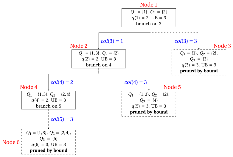
  Node \(1\) is extracted from \(L\). The vertices \(3,5,6,7\) have one colored neighbour each, so \(\mathit{sat}_1=1\); the others have \(\mathit{sat}_1=0\). The four tied vertices have \(\mathit{du}_1=2\), so the smallest index wins: the branching vertex is \(3\). Its neighbour \(2\) has color \(2\), so \(F_1(3)=\{1\}\).

  1. Node \(2\): \(\mathit{col}(3)=1\), with \(q(2)=2<\UB\). The node survives.

  2. Node \(3\): \(\mathit{col}(3)=3\), the new color, with \(q(3)=3\ge\UB\). The node is pruned by bound.

• Iteration 2

  Node \(2\) is extracted from \(L\), with \(Q_1=\{1,3\}\) and \(Q_2=\{2\}\). The vertices \(4,5,6,7,8\) have \(\mathit{sat}_2=1\) and \(\mathit{du}_2=2\), and \(9,10\) have \(\mathit{sat}_2=0\): the branching vertex is \(4\). Its neighbour \(3\) has color \(1\), so \(F_2(4)=\{2\}\).

  1. Node \(4\): \(\mathit{col}(4)=2\), with \(q(4)=2<\UB\). The node survives.

  2. Node \(5\): \(\mathit{col}(4)=3\), with \(q(5)=3\ge\UB\). The node is pruned by bound.

• Iteration 3

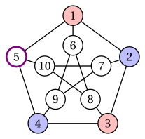
  Node \(4\) is extracted from \(L\), with \(Q_1=\{1,3\}\) and \(Q_2=\{2,4\}\). Vertex \(5\) has the neighbours \(1\) (color \(1\)) and \(4\) (color \(2\)): \(\mathit{sat}_4(5)=2\), the only vertex with saturation degree \(2\), so it is the branching vertex. Its feasible colors are \(F_4(5)=\emptyset\).

  1. Node \(6\): \(\mathit{col}(5)=3\), the only child, with \(q(6)=3\ge\UB\). The node is pruned by bound.

  The partial coloring of node \(4\) is drawn below: the cycle \(1,2,3,4,5\) has five vertices, and two colors are not enough to close it.

  

• Termination

  The list \(L\) is empty: the incumbent solution \(\bar{\mathcal{Q}}\) is optimal and \(\chi(G)=\UB=3\). The tree has \(6\) nodes.

This is the branch-and-bound tree, showing for each node its color classes, the number of colors \(q\), the upper bound \(\UB\) at the moment of the evaluation, and the branching vertex or the pruning criterion. The pruned nodes are dashed.

The nodes in the order of evaluation:

Node	Parent	Child	\(q\)	\(\UB\)	Branching vertex	Outcome
\(1\)	–	root, \(K=\{1,2\}\)	\(2\)	\(3\)	\(3\) (\(\mathit{sat}=1\), \(\mathit{du}=2\))	branched
\(2\)	\(1\)	\(\mathit{col}(3)=1\)	\(2\)	\(3\)	\(4\) (\(\mathit{sat}=1\), \(\mathit{du}=2\))	branched
\(3\)	\(1\)	\(\mathit{col}(3)=3\)	\(3\)	\(3\)	–	pruned by bound
\(4\)	\(2\)	\(\mathit{col}(4)=2\)	\(2\)	\(3\)	\(5\) (\(\mathit{sat}=2\), \(\mathit{du}=1\))	branched
\(5\)	\(2\)	\(\mathit{col}(4)=3\)	\(3\)	\(3\)	–	pruned by bound
\(6\)	\(4\)	\(\mathit{col}(5)=3\)	\(3\)	\(3\)	–	pruned by bound

• The algorithm does not improve the incumbent solution: it proves that \(\UB=3\) is optimal. The proof is the odd cycle \(1,2,3,4,5\), found by the search in three levels.

• Without the pruning, the tree of the Petersen graph has \(9\,776\) nodes and \(7\,430\) leaves, one for each feasible partition counted in Chapter 4, as Proposition 42.2 predicts.

42.3 Remarks

• Origin. The saturation degree and the exact algorithm that branches on it are due to Brélaz (1979). Pre-coloring a clique is the usual way to remove the symmetry of the first colors.

• Sewell's tie-breaking (1996). Among the vertices of maximum saturation degree, Sewell chooses the vertex \(v\) that maximizes the number of feasible colors it shares with its uncolored neighbours, \(\sum_{u\in N(v)\cap U^k} |F_k(v)\cap F_k(u)|\). Coloring that vertex removes the most options from the rest of the graph.

• PASS (San Segundo, 2012). PASS applies Sewell's rule only to selected vertices, computing the count over the vertices tied for the maximum saturation degree, which is cheaper. Both rules change only the tie-breaking: the children, the bounds and Proposition 42.2 stay the same.

• References: D. Brélaz, «New methods to color the vertices of a graph», Communications of the ACM 22(4), 251–256, 1979; E. C. Sewell, «An improved algorithm for exact graph coloring», in D. S. Johnson, M. A. Trick (eds.), Cliques, Coloring, and Satisfiability, DIMACS Series in Discrete Mathematics and Theoretical Computer Science 26, 1996; P. San Segundo, «A new DSATUR-based algorithm for exact vertex coloring», Computers & Operations Research 39(7), 1724–1733, 2012.

42.4 Typical mistakes

Warning

• Counting colored neighbours instead of colors. The saturation degree counts the different colors around \(v\): two neighbours with the same color count once.

• One child per color \(1,\dots,\UB-1\). The unused colors are all equivalent: only the first new color \(q(k)+1\) gives a child, otherwise the tree contains symmetric copies of the same coloring.

• Forgetting the new color. The child with color \(q(k)+1\) is always created, even when \(F_k(v)\neq\emptyset\); without it some colorings are never reached.

• Pruning with \(q(k)>\UB\). A node with \(q(k)=\UB\) cannot lead to a better coloring, because the number of colors is an integer: the rule is \(q(k)\ge\UB\).

• Pre-coloring a set that is not a clique. Only the vertices of a clique need pairwise different colors in every coloring; pre-coloring two non-adjacent vertices with different colors can cut off all the optimal colorings.

• Continuing after \(\UB=|K|\). When a complete coloring reaches the clique bound, it is optimal: the nodes still in the list are not explored.

42.5 In summary

In summary

• A node of the DSATUR branch-and-bound is a partial coloring; the algorithm branches on the most saturated vertex, with one child per feasible color and one new color.

• \(DSATUR\) gives the first upper bound, a greedy clique gives the lower bound and is pre-colored; a node is pruned when \(q(k)\ge\UB\).

• Without pruning the tree enumerates every feasible coloring once, up to a renaming of the colors: the algorithm is exact.

Dashboard of the Petersen graph (\(n=10\), \(m=15\)). The bounds on \(\chi(G)\) found so far:

Source	Lower bound	Upper bound	From
Clique bound (Chapter 4)	\(2\)	–	\(\omega(G)=2\)
\(DSATUR\) (Chapter 30)	–	\(3\)	\(\{1,3,7\}\), \(\{2,4,6,10\}\), \(\{5,8,9\}\)
This chapter, initialization	\(2\)	\(3\)	greedy clique \(K=\{1,2\}\)
This chapter, termination	\(3\)	\(3\)	empty list, \(6\) nodes

---

Exercises on this chapter: Vertex coloring (VCP)

In the interactive lab: Vertex coloring: the DSATUR branch-and-bound.