DP for the coin change problem¶

Part 3 · Dynamic programming · Chapter 27 · Lecture notes, volume 3 (PDF) · Slides · Exercises: Coin change (CCP)

Prerequisites

From this module, the chapter «DP for the unbounded knapsack problem»: unlimited supply of every item type, and the reconstruction of a solution.
From this module, the chapter «Principles of dynamic programming»: optimal substructure, overlapping subproblems, base cases.
From the module Algorithms: pseudocode conventions (Chapter 2) and the size of the input (Chapter 11).

Objectives

At the end of this chapter you will be able to:

explain why the CCP asks for an exact amount and why an instance can be infeasible;
write the recurrence $v(k)$ with the value $+\infty$ for the amounts that cannot be returned;
run the DP algorithm by hand, following the comparisons with the running best value $m$;
reconstruct an optimal solution as the vector $(x_1,\dots,x_n)$ when the instance is feasible;
count the steps of the DP algorithm.

The problem of this chapter is the coin change problem (CCP): its definition is on its page.

27.1 Instances and feasible solutions¶

Example 27.1: CCP instance

We consider an amount of change $c=10$ to return, and $n=3$ denominations:

\[ w = (2,3,5). \]

We refer to this CCP instance as Example 27.1.

Unlike the 0/1 knapsack problem (KP), where the total weight of the selected items must not exceed the capacity, the CCP requires the total value of the selected coins to be exactly equal to $c$. Moreover, since every denomination is available in unlimited supply, the number of coins of a given denomination used in a solution is not bounded a priori.

27.1.1 Encoding of feasible solutions¶

A feasible solution of the CCP is a choice of the number of coins of each denomination whose total value is exactly equal to the amount of change $c$.

A CCP feasible solution can be described by the integer vector

\[ (x_1,x_2,\dots,x_n) \]

where each component has the following meaning:

\[ x_j = \text{number of coins of denomination } j \text{ used}, \qquad \forall j \in \{1,2,\dots,n\}, \quad x_j \in \Z_{\ge 0}. \]

Since the solution is feasible, the total value of the selected coins must be exactly equal to $c$:

\[ \sum_{j=1}^{n} w_j x_j = c. \]

The total number of coins of a feasible solution is

\[ \sum_{j=1}^{n} x_j. \]
Since $\sum_{j=1}^{n} w_j x_j = c$, every component $x_j$ of a feasible solution satisfies $x_j \le \lfloor c/w_j \rfloor$. Therefore, the number of feasible solutions is finite, but it grows quickly with $c$ and $n$, and enumerating all of them to find the one using the fewest coins quickly becomes impractical.

27.2 A DP algorithm¶

Step 1: computation of the optimal value

For any $k \in \{0,1,\dots,c\}$, let $v(k)$ be the optimal value of the CCP subinstance given by:

an integer amount of change $k$ to return,
the same set $\{1,2,\dots,n\}$ of denominations, each available in unlimited supply.

The recursive formula to compute $v(k)$ reads as follows:

\[\begin{equation*} \label{eq:ccp} v(k)= \left\{ \begin{array}{ll} 0 & \textrm{if $k=0$,} \\[2ex] +\infty & \textrm{if $k\ge 1$ and $w_j>k$ for every $j\in\{1,2,\dots,n\}$,} \\[2ex] \displaystyle \min_{j \,:\, w_j \,\le\, k} \big\{ 1 + v(k-w_j) \big\} & \textrm{if $k\ge 1$ and $w_j\le k$ for some $j\in\{1,2,\dots,n\}$.} \end{array} \right. \tag{27.1} \end{equation*}\]

The recursive decomposition process of formula $\eqref{eq:ccp}$ generates at most $n$ independent subproblems, corresponding to the possible choices of a denomination $j$, with $w_j\le k$, used as one of the coins returning the amount of change $k$.
The base case is $v(0)=0$ since no coin is needed to return a null amount of change, and $v(k)=+\infty$ if no denomination is small enough to be used, since in this case the amount of change $k$ cannot be returned at all.
The optimal value $v(k)$ is obtained by trying every denomination $j$ with $w_j\le k$ and selecting the one that minimizes the sum $1+v(k-w_j)$ of the single coin of denomination $j$ and the optimal value of the residual subproblem, returning the remaining amount of change $k-w_j$.
Hence, an optimal solution for the subinstance with amount of change $k$ is built by combining the chosen coin of denomination $j$ with an optimal solution of the corresponding residual subproblem, returning the amount of change $k-w_j$.

$\rightsquigarrow$ Optimal Substructure verified!
Different choices of the denomination used as the first coin, possibly made for different values of $k$, can lead to the same residual amount of change, and therefore the same value $v(k)$ may need to be computed several times during the recursive evaluation of formula $\eqref{eq:ccp}$.

$\rightsquigarrow$ Overlapping Subproblems verified!
A first method to compute the optimal value $v(c)$ of the CCP instance is the top-down approach. The method starts from the call with $k=c$ and evaluates formula $\eqref{eq:ccp}$ recursively: each call tries every denomination $j$ with $w_j\le k$, until the amount of change is equal to $0$ or no denomination is small enough to be used.
The recursion tree of the function $v$ has one node for each recursive call, labeled with the function call it represents. The root represents the initial call. The children of a node represent the recursive calls made by that call. The leaf nodes represent the base cases.

Example 27.2: Recursion tree

We consider the CCP instance of Example 27.1. This is the recursion tree of the top-down approach to compute $v(10)$:

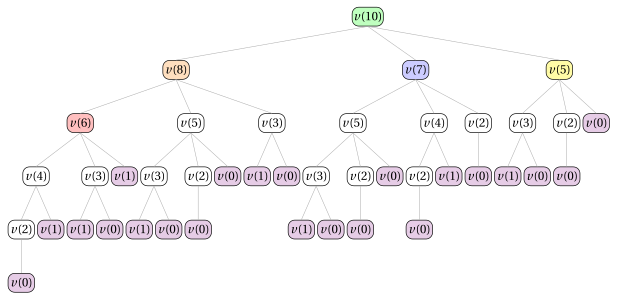
The function $v$ is called $42$ times, and the same subproblems are solved multiple times: $v(0)$ is called $14$ times, $v(1)$ is called $8$ times, $v(2)$ is called $6$ times, $v(3)$ is called $5$ times, $v(4)$ is called $2$ times, and $v(5)$ is called $3$ times. All the other calls are made only once.
The value $v(k)$ can be computed once the values $v(k')$, for every smaller amount of change $k'<k$, are known. Therefore, all values $v(k)$ can be computed by considering the amount of change $k$ in increasing order.
Example 27.3: Computing the values of the $v$ function

We consider the CCP instance of Example 27.1, with amount of change $c=10$ to return and denominations $w=(2,3,5)$.

The values of the function $v$ are computed as follows:
- The base case gives $v(0)=0$.
- Once we have computed $v(0)$, we can compute $v(1)$: since no denomination satisfies $w_j\le 1$, we obtain
  
  \[ v(1) = +\infty. \]
- Once we have computed $v(0)$, we can compute $v(2)$:
  
  \[ v(2) = 1+v(0) = 1+0 = 1. \]
- Once we have computed $v(0)$ and $v(1)$, we can compute $v(3)$:
  
  \[ v(3) = \min\{1+v(1),\,1+v(0)\} = \min\{1+\infty,\,1+0\} = 1. \]
- Once we have computed $v(1)$ and $v(2)$, we can compute $v(4)$, trying every denomination $j$ with $w_j\le 4$:
  
  \[ v(4) = \min\{1+v(2),\,1+v(1)\} = \min\{1+1,\,1+\infty\} = 2. \]
- Once we have computed $v(0)$, $v(2)$, and $v(3)$, we can compute $v(5)$:
  
  \[ v(5) = \min\{1+v(3),\,1+v(2),\,1+v(0)\} = \min\{1+1,\,1+1,\,1+0\} = 1. \]
- Once we have computed $v(1)$, $v(3)$, and $v(4)$, we can compute $v(6)$:
  
  \[ v(6) = \min\{1+v(4),\,1+v(3),\,1+v(1)\} = \min\{1+2,\,1+1,\,1+\infty\} = 2. \]
- Once we have computed $v(2)$, $v(4)$, and $v(5)$, we can compute $v(7)$, trying every denomination $j$ with $w_j\le 7$:
  
  \[ v(7) = \min\{1+v(5),\,1+v(4),\,1+v(2)\} = \min\{1+1,\,1+2,\,1+1\} = 2. \]
  
  Here, the denominations $w_1=2$ and $w_3=5$ are tied: both give value $2$. Since the bottom-up algorithm only updates the optimal value when a strictly smaller value is found, the first denomination achieving the minimum, $w_1=2$, is the one recorded.
- Once we have computed $v(3)$, $v(5)$, and $v(6)$, we can compute $v(8)$:
  
  \[ v(8) = \min\{1+v(6),\,1+v(5),\,1+v(3)\} = \min\{1+2,\,1+1,\,1+1\} = 2. \]
- Finally, once we have computed $v(5)$, $v(7)$, and $v(8)$, we can compute $v(10)$, trying every denomination $j$ with $w_j\le 10$:
  
  \[ v(10) = \min\{1+v(8),\,1+v(7),\,1+v(5)\} = \min\{1+2,\,1+2,\,1+1\} = 2. \]
We can avoid solving the same subproblems repeatedly by storing the value of each subproblem as soon as it is computed. The values are stored in a lookup table.
Since solving any particular subproblem depends only on subproblems with a smaller amount of change, we can solve the subproblems in increasing order of $k$, starting from the base case $v(0)=0$ and building up to $v(c)$.
This observation naturally leads to a much more efficient method to compute the optimal value $v(c)$ of the CCP instance.

A second method to compute the optimal value $v(c)$ of the CCP instance is the bottom-up approach. The method starts from the base case and evaluates formula $\eqref{eq:ccp}$ for increasing values of $k \in \{1,2,\dots,c\}$: each value $v(k)$ is computed using already-computed values, until the value $v(c)$ of the CCP instance is obtained.

This is the pseudo-code of the DP algorithm using the bottom-up approach:

Algorithm: CCP_DP

Input: A CCP instance given by $n$, the array $w[1..n]$ of denominations, and the amount of change $c$

Output: The optimal value

1Function CCP_DP($n,w,c$)

2$v := \textnormal{new array}[0..c]$

3$v[0] \leftarrow 0$

4for $k := 1$ to $c$ do

5$m := +\infty$

6for $j := 1$ to $n$ do

7if $w[j]\le k$ and $1+v[k-w[j]] < m$ then

8$m \leftarrow 1+v[k-w[j]]$

9end

10end

11$v[k] \leftarrow m$

12end

13return $v[c]$

The array $v[0..c]$ is the lookup table: it stores the optimal values of all subproblems.
The instruction $v[0] \leftarrow 0$ initializes the base case, corresponding to a null amount of change.
The outer loop, over $k \in \{1,2,\dots,c\}$, computes the entries of the array in increasing order of amount of change.
The inner loop, over $j \in \{1,2,\dots,n\}$, tries every denomination and keeps in $m$ the smallest value found so far; $m$ is initialized to $+\infty$, so that $v[k]$ remains $+\infty$ if no denomination $j$ with $w[j]\le k$ is found.
At the end of the inner loop, $v[k] \leftarrow m$ stores the optimal value $v[k]$.
Finally, the optimal value of the CCP instance is returned as $v[c]$.

Example 27.4: Execution of the DP algorithm

We consider the CCP instance of Example 27.1, with amount of change $c=10$ to return and denominations $w=(2,3,5)$.

For each step of the DP algorithm, the table shows the values of $k$ and $j$, the cell $v[k]$, the current value of $m$, and the comparison performed. The cell of $m$ is highlighted in red when updated; the cell of $v[k]$ is highlighted in blue when assigned.

$k$	$j$	$v[k]$	$m$	Action
$-$	$-$	0	$-$	$v[0]\leftarrow 0$
	$-$	$-$	$+\infty$	$m := +\infty$
1	1	$-$	$+\infty$	$w[1]=2>1$: skip
	2	$-$	$+\infty$	$w[2]=3>1$: skip
	3	$-$	$+\infty$	$w[3]=5>1$: skip
	$-$	$+\infty$	$+\infty$	$v[1]\leftarrow m=+\infty$
	$-$	$-$	$+\infty$	$m := +\infty$
2	1	$-$	$1$	$1{+}v[0]=1<m$: $m\leftarrow 1$
	2	$-$	$1$	$w[2]=3>2$: skip
	3	$-$	$1$	$w[3]=5>2$: skip
	$-$	$1$	$1$	$v[2]\leftarrow m=1$
	$-$	$-$	$+\infty$	$m := +\infty$
3	1	$-$	$+\infty$	$1{+}v[1]=+\infty\not<m=+\infty$: no update
	2	$-$	$1$	$1{+}v[0]=1<m$: $m\leftarrow 1$
	3	$-$	$1$	$w[3]=5>3$: skip
	$-$	$1$	$1$	$v[3]\leftarrow m=1$
	$-$	$-$	$+\infty$	$m := +\infty$
4	1	$-$	$2$	$1{+}v[2]=2<m$: $m\leftarrow 2$
	2	$-$	$2$	$1{+}v[1]=+\infty\not<m=2$: no update
	3	$-$	$2$	$w[3]=5>4$: skip
	$-$	$2$	$2$	$v[4]\leftarrow m=2$
	$-$	$-$	$+\infty$	$m := +\infty$
5	1	$-$	$2$	$1{+}v[3]=2<m$: $m\leftarrow 2$
	2	$-$	$2$	$1{+}v[2]=2\not<m=2$: no update
	3	$-$	$1$	$1{+}v[0]=1<m$: $m\leftarrow 1$
	$-$	$1$	$1$	$v[5]\leftarrow m=1$
	$-$	$-$	$+\infty$	$m := +\infty$
6	1	$-$	$3$	$1{+}v[4]=3<m$: $m\leftarrow 3$
	2	$-$	$2$	$1{+}v[3]=2<m$: $m\leftarrow 2$
	3	$-$	$2$	$1{+}v[1]=+\infty\not<m=2$: no update
	$-$	$2$	$2$	$v[6]\leftarrow m=2$
	$-$	$-$	$+\infty$	$m := +\infty$
7	1	$-$	$2$	$1{+}v[5]=2<m$: $m\leftarrow 2$
	2	$-$	$2$	$1{+}v[4]=3\not<m=2$: no update
	3	$-$	$2$	$1{+}v[2]=2\not<m=2$: no update
	$-$	$2$	$2$	$v[7]\leftarrow m=2$
	$-$	$-$	$+\infty$	$m := +\infty$
8	1	$-$	$3$	$1{+}v[6]=3<m$: $m\leftarrow 3$
	2	$-$	$2$	$1{+}v[5]=2<m$: $m\leftarrow 2$
	3	$-$	$2$	$1{+}v[3]=2\not<m=2$: no update
	$-$	$2$	$2$	$v[8]\leftarrow m=2$
	$-$	$-$	$+\infty$	$m := +\infty$
9	1	$-$	$3$	$1{+}v[7]=3<m$: $m\leftarrow 3$
	2	$-$	$3$	$1{+}v[6]=3\not<m=3$: no update
	3	$-$	$3$	$1{+}v[4]=3\not<m=3$: no update
	$-$	$3$	$3$	$v[9]\leftarrow m=3$
	$-$	$-$	$+\infty$	$m := +\infty$
10	1	$-$	$3$	$1{+}v[8]=3<m$: $m\leftarrow 3$
	2	$-$	$3$	$1{+}v[7]=3\not<m=3$: no update
	3	$-$	$2$	$1{+}v[5]=2<m$: $m\leftarrow 2$
	$-$	$2$	$2$	$v[10]\leftarrow m=2$

This is the array $v$ after the execution of the DP algorithm:

\[ \begin{array}{l|rrrrrrrrrrr} \hline {k} & 0 & 1 & 2 & 3 & 4 & 5 & 6 & 7 & 8 & 9 & 10 \\ \hline {v[k]} & 0 & {+\infty} & 1 & 1 & 2 & 1 & 2 & 2 & 2 & 3 & 2 \\ \hline \end{array} \]

After the execution of the DP algorithm, the array $v$ contains the optimal value $v[k]$ for every amount of change $k \in \{0,1,\dots,c\}$, where $v[c]$ is the minimum number of coins needed to return the amount of change $c$.

Step 2: computation of an optimal solution
- To compute an optimal solution, i.e., the integer vector $(x_1,x_2,\dots,x_n)$, it is necessary to store some additional information.
- For each amount of change $k$, in addition to the optimal value $v[k]$, we store $s[k]$, the index of the denomination of the coin used to obtain the optimal value $v[k]$ in formula $\eqref{eq:ccp}$.
- More precisely, $s[k]$ is equal to the index $j$ of the denomination $w_j$ that minimizes the right-hand side of formula $\eqref{eq:ccp}$ when computing $v[k]$.
  
  This is the pseudo-code of the DP algorithm using the bottom-up approach with the storing of the information necessary to construct an optimal solution:
  
  Algorithm: CCP_DP_InfoSol
  
  Input: A CCP instance given by $n$, the array $w[1..n]$ of denominations, and the amount of change $c$
  Output: The optimal value and the array $s[0..c]$ of the indices of the denominations used
  1Function CCP_DP_InfoSol($n,w,c$)
  2$v := \textnormal{new array}[0..c]$; $s := \textnormal{new array}[0..c]$
  3$v[0] \leftarrow 0$; $s[0] \leftarrow 0$
  4for $k := 1$ to $c$ do
  5$m := +\infty$; $t := 0$
  6for $j := 1$ to $n$ do
  7if $w[j]\le k$ and $1+v[k-w[j]] < m$ then
  8$m \leftarrow 1+v[k-w[j]]$; $t \leftarrow j$
  9end
  10end
  11$v[k] \leftarrow m$; $s[k] \leftarrow t$
  12end
  13return $v[c], s$
  - The DP algorithm uses the additional temporary variable $t$ to keep track of the decision made when $m$ is updated. If the denomination $w[j]$ is used, $t \leftarrow j$ stores its index. At the end of the inner loop, $s[k]\leftarrow t$ stores the index of the denomination of the coin used, together with the optimal value $v[k]\leftarrow m$.
  Example 27.5: Computation of the additional information
  
  We consider the CCP instance of Example 27.1, with amount of change $c=10$ to return and denominations $w=(2,3,5)$.
  
  This is the array $s$ after the execution of the DP algorithm:
  
  \[ \begin{array}{l|rrrrrrrrrrr} \hline {k} & 0 & 1 & 2 & 3 & 4 & 5 & 6 & 7 & 8 & 9 & 10 \\ \hline {s[k]} & 0 & 0 & 1 & 2 & 1 & 3 & 2 & 1 & 2 & 1 & 3 \\ \hline \end{array} \]
  
  For example, $s[5]=3$ since formula $\eqref{eq:ccp}$ selects the denomination $w_3=5$ when computing $v[5]=1$, and $s[10]=3$ since the denomination $w_3=5$ is also selected when computing $v[10]=2$. The entry $s[1]$ is left undefined ($0$, by convention), since $v[1]=+\infty$ is infeasible.
- Once the array $s$ has been computed, and provided that $v[c]<+\infty$, an optimal solution can be reconstructed by repeatedly using one coin of denomination $s[k]$ and moving to the residual amount of change $k-w_{s[k]}$, starting from $k=c$ and $x_j=0$ for all $j \in \{1,2,\dots,n\}$, until $k=0$:
  
  \[ x_{s[k]} \leftarrow x_{s[k]}+1, \qquad k \leftarrow k - w_{s[k]}. \]
  
  This yields the vector $(x_1,x_2,\dots,x_n)$, where each entry $x_j$ is the number of coins of denomination $j$ in an optimal solution.
- The condition $v[c]<+\infty$ is necessary: if $v[c]=+\infty$ the instance is infeasible, $s[c]=0$ and there is no solution to reconstruct. If $v[c]<+\infty$, then $s[k]\ge 1$ for every amount of change $k$ visited by the procedure.
  
  Algorithm: CCP_Reconstruct
  
  Input: The number $n$ of denominations, the array $w[1..n]$, the amount of change $c$ with $v[c]<+\infty$, and the array $s[0..c]$
  Output: An optimal solution
  1Function CCP_Reconstruct($n,w,c,s$)
  2$x := \textnormal{new array}[1..n]$
  3for $j := 1$ to $n$ do
  4$x[j] \leftarrow 0$
  5end
  6$k := c$
  7while $k>0$ do
  8$x[s[k]] \leftarrow x[s[k]]+1$
  9$k \leftarrow k-w[s[k]]$
  10end
  11return $x$
  
  Example 27.6: Computing an optimal solution
  
  After the execution of the DP algorithm on the instance of Example 27.1, we have the following array $s$:
  
  \[ \begin{array}{l|rrrrrrrrrrr} \hline {k} & 0 & 1 & 2 & 3 & 4 & 5 & 6 & 7 & 8 & 9 & 10 \\ \hline {s[k]} & 0 & 0 & 1 & 2 & 1 & 3 & 2 & 1 & 2 & 1 & 3 \\ \hline \end{array} \]
  
  We can reconstruct an optimal solution by starting from $k=10$ as follows:
  
  Iteration $k$ $s[k]$ $x[1]$ $x[2]$ $x[3]$ $k \leftarrow k-w_{s[k]}$
  
  $-$ $-$ $-$ 0 0 0 $k=10$
  
  $1$ $10$ $3$ 0 0 1 $k=10-5=5$
  
  $2$ $5$ $3$ 0 0 2 $k=5-5=0$
  
  Thus, the vector
  
  \[ (0,0,2) \]
  
  is an optimal solution: it uses two coins of denomination $w_3=5$. The corresponding total value is $2\cdot5=10=c$. The corresponding optimal value is $v(10)=2$.

27.2.1 Number of steps¶

Let $S(n,c)$ denote the number of steps executed by CCP_DP in the worst case, where $n$ is the number of denominations and $c$ is the amount of change. We compute $S(n,c)$ by counting how many times the lines of the pseudo-code of CCP_DP are executed.
In the worst case, the condition at line 7 is true at every iteration of the inner loop, and therefore line 8 is executed as often as line 7. The number of executions of the relevant lines is:
- Line 2 is executed $1$ time.
- Line 3 is executed $1$ time.
- Line 4 is executed $c$ times.
- Line 5 is executed $c$ times.
- Line 6 is executed $cn$ times.
- Line 7 is executed $cn$ times.
- Line 8 is executed $cn$ times.
- Line 11 is executed $c$ times.
- Line 13 is executed $1$ time.
Therefore, the total number of steps in the worst case is

\[ 1+1+c+c+cn+cn+cn+c+1. \]

Thus,

\[ S(n,c)=3+3c+3cn. \]

Hence,

\[ S(n,c)=\Theta(nc). \]

Indeed,

\[ \lim_{n,c\to\infty} \frac{3cn+3c+3}{nc} = \lim_{n,c\to\infty} \left(3+\frac{3}{n}+\frac{3}{nc}\right) = 3\in\mathbb{R}_{>0}. \]

The DP algorithm executes

\[ S(n,c)=\Theta(nc) \]

steps in the worst case.
The version CCP_DP_InfoSol stores the additional array $s$ and performs only a constant number of extra operations inside the same loops. Therefore, its number of steps remains $\Theta(nc)$.

27.3 Typical mistakes¶

Warning

Using $0$ instead of $+\infty$. An amount that cannot be returned has $v(k)=+\infty$; with the value $0$ the DP algorithm would claim that no coin is needed.
Reconstructing an infeasible instance. If $v[c]=+\infty$ then $s[c]=0$, and the reconstruction would read $x[0]$ and $w[0]$, outside the arrays: it must first check that $v[c]<+\infty$.
Storing the value of the coin instead of its index. The vector $x$ is indexed by the denominations: $s[k]$ stores the index $j$, and the coin value is $w_{s[k]}$.
Confusing the CCP with the UKP. The CCP asks for exactly $c$ and minimizes the number of coins; the UKP asks for at most $c$ and maximizes the profit.

27.4 In summary¶

In summary

The CCP asks for the minimum number of coins whose total value is exactly $c$; the instance is infeasible when $v(c)=+\infty$.
The recurrence $v(k)=\min_{j:\,w_j\le k}\{1+v(k-w_j)\}$ is computed bottom-up in $\Theta(nc)$ steps, which is pseudo-polynomial.
An optimal solution is read backwards from $s[c]$, the index of the denomination of the first coin chosen for the amount $c$, and only if $v[c]<+\infty$.

Dashboard of the CCP example. Example 27.1 ($c=10$, $w=(2,3,5)$):

Method	Lower bound	Upper bound	Origin
DP algorithm	$2$	$2$	minimum number of coins, solution $(0,0,2)$

Exercises on this chapter: Coin change (CCP)

\(k\)	\(j\)	\(v[k]\)	\(m\)	Action
\(-\)	\(-\)	0	\(-\)	\(v[0]\leftarrow 0\)
	\(-\)	\(-\)	\(+\infty\)	\(m := +\infty\)
1	1	\(-\)	\(+\infty\)	\(w[1]=2>1\): skip
	2	\(-\)	\(+\infty\)	\(w[2]=3>1\): skip
	3	\(-\)	\(+\infty\)	\(w[3]=5>1\): skip
	\(-\)	\(+\infty\)	\(+\infty\)	\(v[1]\leftarrow m=+\infty\)
	\(-\)	\(-\)	\(+\infty\)	\(m := +\infty\)
2	1	\(-\)	\(1\)	\(1{+}v[0]=1<m\): \(m\leftarrow 1\)
	2	\(-\)	\(1\)	\(w[2]=3>2\): skip
	3	\(-\)	\(1\)	\(w[3]=5>2\): skip
	\(-\)	\(1\)	\(1\)	\(v[2]\leftarrow m=1\)
	\(-\)	\(-\)	\(+\infty\)	\(m := +\infty\)
3	1	\(-\)	\(+\infty\)	\(1{+}v[1]=+\infty\not<m=+\infty\): no update
	2	\(-\)	\(1\)	\(1{+}v[0]=1<m\): \(m\leftarrow 1\)
	3	\(-\)	\(1\)	\(w[3]=5>3\): skip
	\(-\)	\(1\)	\(1\)	\(v[3]\leftarrow m=1\)
	\(-\)	\(-\)	\(+\infty\)	\(m := +\infty\)
4	1	\(-\)	\(2\)	\(1{+}v[2]=2<m\): \(m\leftarrow 2\)
	2	\(-\)	\(2\)	\(1{+}v[1]=+\infty\not<m=2\): no update
	3	\(-\)	\(2\)	\(w[3]=5>4\): skip
	\(-\)	\(2\)	\(2\)	\(v[4]\leftarrow m=2\)
	\(-\)	\(-\)	\(+\infty\)	\(m := +\infty\)
5	1	\(-\)	\(2\)	\(1{+}v[3]=2<m\): \(m\leftarrow 2\)
	2	\(-\)	\(2\)	\(1{+}v[2]=2\not<m=2\): no update
	3	\(-\)	\(1\)	\(1{+}v[0]=1<m\): \(m\leftarrow 1\)
	\(-\)	\(1\)	\(1\)	\(v[5]\leftarrow m=1\)
	\(-\)	\(-\)	\(+\infty\)	\(m := +\infty\)
6	1	\(-\)	\(3\)	\(1{+}v[4]=3<m\): \(m\leftarrow 3\)
	2	\(-\)	\(2\)	\(1{+}v[3]=2<m\): \(m\leftarrow 2\)
	3	\(-\)	\(2\)	\(1{+}v[1]=+\infty\not<m=2\): no update
	\(-\)	\(2\)	\(2\)	\(v[6]\leftarrow m=2\)
	\(-\)	\(-\)	\(+\infty\)	\(m := +\infty\)
7	1	\(-\)	\(2\)	\(1{+}v[5]=2<m\): \(m\leftarrow 2\)
	2	\(-\)	\(2\)	\(1{+}v[4]=3\not<m=2\): no update
	3	\(-\)	\(2\)	\(1{+}v[2]=2\not<m=2\): no update
	\(-\)	\(2\)	\(2\)	\(v[7]\leftarrow m=2\)
	\(-\)	\(-\)	\(+\infty\)	\(m := +\infty\)
8	1	\(-\)	\(3\)	\(1{+}v[6]=3<m\): \(m\leftarrow 3\)
	2	\(-\)	\(2\)	\(1{+}v[5]=2<m\): \(m\leftarrow 2\)
	3	\(-\)	\(2\)	\(1{+}v[3]=2\not<m=2\): no update
	\(-\)	\(2\)	\(2\)	\(v[8]\leftarrow m=2\)
	\(-\)	\(-\)	\(+\infty\)	\(m := +\infty\)
9	1	\(-\)	\(3\)	\(1{+}v[7]=3<m\): \(m\leftarrow 3\)
	2	\(-\)	\(3\)	\(1{+}v[6]=3\not<m=3\): no update
	3	\(-\)	\(3\)	\(1{+}v[4]=3\not<m=3\): no update
	\(-\)	\(3\)	\(3\)	\(v[9]\leftarrow m=3\)
	\(-\)	\(-\)	\(+\infty\)	\(m := +\infty\)
10	1	\(-\)	\(3\)	\(1{+}v[8]=3<m\): \(m\leftarrow 3\)
	2	\(-\)	\(3\)	\(1{+}v[7]=3\not<m=3\): no update
	3	\(-\)	\(2\)	\(1{+}v[5]=2<m\): \(m\leftarrow 2\)
	\(-\)	\(2\)	\(2\)	\(v[10]\leftarrow m=2\)

Iteration	\(k\)	\(s[k]\)	\(x[3]\)	\(k \leftarrow k-w_{s[k]}\)
\(-\)	\(-\)	\(-\)	0	\(k=10\)
\(1\)	\(10\)	\(3\)	1	\(k=10-5=5\)
\(2\)	\(5\)	\(3\)	2	\(k=5-5=0\)