31.7 TSP: 2-opt and Or-opt
Part 4 · Heuristic algorithms · Chapter 31 · Chapter 31: Local search · Lecture notes, volume 4 (PDF) · Slides (1/2) · Slides (2/2) · Exercises: Local search · App: TSP: nearest neighbour and 2-opt
31.7.1 The 2-opt local search
The 2-opt local search (denoted by \(2OPT\)) is a local search for the TSP with the 2-opt neighbourhood. At every iteration it evaluates the 2-opt moves of the current tour with the incremental formula, applies an improving move chosen by the first- or the best-improvement rule, and stops when no move shortens the tour.
Algorithm: 2-opt step
-
In the implementation, \(\textit{Improve}\) and the move to the improving neighbour are merged in a single function \(\textit{Step}\), which explores the neighbourhood with the incremental evaluation and, if it finds an improving move, applies it to the current solution and returns true; otherwise it returns false. \(LS\) calls \(\textit{Step}\) until it returns false.
-
\(2OPT\) is \(\textit{LocalSearch}\) with \(\textit{TwoOptStep}\); it never changes \(\sigma[1]=1\), since \(i\ge 1\) and the reversed path starts at position \(i+1\ge 2\).
-
An iteration costs \(O(n^2)\) time; the reversal of the path costs \(O(n)\).
-
When the distances are Euclidean, a 2-opt local optimum has no crossing edges: if the edges \(\{u_1,v_1\}\) and \(\{u_2,v_2\}\) cross at a point \(X\), the triangle inequality gives \(d_{u_1u_2}\le d_{u_1X}+d_{Xu_2}\) and \(d_{v_1v_2}\le d_{v_1X}+d_{Xv_2}\), so \(\Delta\le 0\), with \(\Delta<0\) unless the four cities are on a line. The 2-opt move “uncrosses” the two edges.
Example 31.2: \(2OPT\) on the TSP reference instance
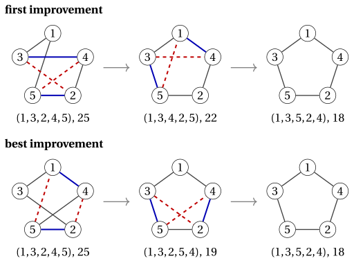
We start from the tour of \(NN\) from city \(1\), \(\sigma=(1,3,2,4,5)\), of length \(25\). Its \(5\) moves are
| \((i,j)\) | removed edges | added edges | \(\Delta\) | new tour, length |
|---|---|---|---|---|
| \((1,3)\) | \(\{1,3\},\{2,4\}\) | \(\{1,2\},\{3,4\}\) | \(5+4-2-3=+4\) | \((1,2,3,4,5)\), \(29\) |
| \((1,4)\) | \(\{1,3\},\{4,5\}\) | \(\{1,4\},\{3,5\}\) | \(2+7-2-7=0\) | \((1,4,2,3,5)\), \(25\) |
| \((2,4)\) | \(\{3,2\},\{4,5\}\) | \(\{3,4\},\{2,5\}\) | \(4+4-4-7=-3\) | \((1,3,4,2,5)\), \(22\) |
| \((2,5)\) | \(\{3,2\},\{5,1\}\) | \(\{3,5\},\{2,1\}\) | \(7+5-4-9=-1\) | \((1,3,5,4,2)\), \(24\) |
| \((3,5)\) | \(\{2,4\},\{5,1\}\) | \(\{2,5\},\{4,1\}\) | \(4+2-3-9=-6\) | \((1,3,2,5,4)\), \(19\) |
First improvement accepts the move \((2,4)\), the first with \(\Delta<0\), after \(3\) evaluations: \(\sigma=(1,3,4,2,5)\), of length \(22\). Its moves have \(\Delta=+1,+6,+3,-4,0\); the move \((2,5)\), which removes \(\{3,4\}\) and \(\{5,1\}\) and adds \(\{3,5\}\) and \(\{4,1\}\), is accepted after \(4\) evaluations: \(\sigma=(1,3,5,2,4)\), of length \(18\). All its \(5\) moves have \(\Delta>0\) (\(+7,+4,+1,+4,+6\)): the search stops after \(3+4+5=12\) evaluations.
Best improvement accepts the move \((3,5)\), with \(\Delta=-6\): \(\sigma=(1,3,2,5,4)\), of length \(19\). Its moves have \(\Delta=+6,+4,-1,+3,+6\), and the move \((2,4)\), which removes \(\{3,2\}\) and \(\{5,4\}\) and adds \(\{3,5\}\) and \(\{2,4\}\), gives \(\sigma=(1,3,5,2,4)\), of length \(18\). The search stops after \(5+5+5=15\) evaluations.
Both rules reach the optimal tour, with \(2\) moves each. The figure shows the two paths; the cities are placed in the order of the optimal tour, so the optimal tour is the boundary of the pentagon (the instance is not Euclidean: the drawing is only a schematic). Dashed red edges are removed, blue edges are added.
31.7.2 The Or-opt local search
The Or-opt local search (denoted by \(OROPT\)) is a local search for the TSP with the Or-opt neighbourhood. At every iteration it evaluates, with the incremental formula, the insertion of every segment of \(1\), \(2\) or \(3\) consecutive cities between two other consecutive cities, applies an improving move chosen by the first- or the best-improvement rule, and stops when no move shortens the tour.
Algorithm: Or-opt step
-
Or-opt moves a short piece of the tour to a better place, without reversing anything: it is the natural neighbourhood when a few cities have been “left behind” by the construction. An iteration costs \(O(n^2)\) time.
-
A 2-opt local optimum need not be an Or-opt local optimum, and vice versa: the two neighbourhoods contain different moves.
31.7.3 First and best improvement on a medium instance
- On \(5\) cities the 2-opt neighbourhood is small and both rules reach the optimum. To see the difference between the two rules, and the role of Or-opt, we use a medium instance with \(10\) cities. This instance is not metric: \(d_{68}=8>d_{67}+d_{78}=4+3\) and \(d_{6,10}=11>d_{67}+d_{7,10}=4+6\).
Example 31.3: A TSP instance with \(10\) cities
The cities have integer coordinates, and \(d_{ij}\) is the Euclidean distance rounded to the nearest integer:
| city | \(1\) | \(2\) | \(3\) | \(4\) | \(5\) | \(6\) | \(7\) | \(8\) | \(9\) | \(10\) |
|---|---|---|---|---|---|---|---|---|---|---|
| coordinates | \((1,1)\) | \((3,8)\) | \((6,10)\) | \((10,9)\) | \((13,6)\) | \((12,1)\) | \((8,3)\) | \((5,4)\) | \((8,7)\) | \((2,5)\) |
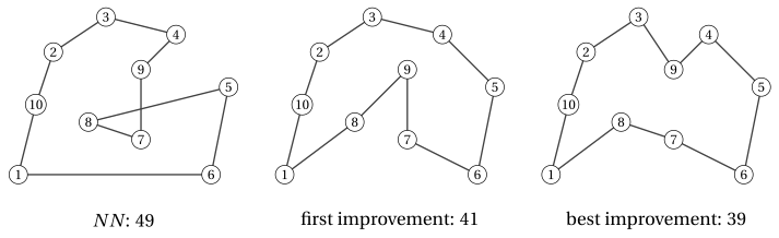
Among its \(181\,440\) distinct tours, the unique optimal one is \((1,10,2,3,9,4,5,6,7,8)\), of length \(z(I)=39\). The tour of \(NN\) from city \(1\) is \((1,10,2,3,4,9,7,8,5,6)\), of length \(49\), and the 2-opt neighbourhood has \(\frac{10\cdot 7}{2}=35\) moves.
First improvement makes \(4\) moves:
| removed edges | new tour | \(\Delta\) | length | evaluations |
|---|---|---|---|---|
| \(\{3,4\},\{8,5\}\) | \((1,10,2,3,8,7,9,4,5,6)\) | \(-2\) | \(47\) | \(23\) |
| \(\{3,8\},\{6,1\}\) | \((1,10,2,3,6,5,4,9,7,8)\) | \(-1\) | \(46\) | \(25\) |
| \(\{3,6\},\{4,9\}\) | \((1,10,2,3,4,5,6,9,7,8)\) | \(-3\) | \(43\) | \(22\) |
| \(\{6,9\},\{7,8\}\) | \((1,10,2,3,4,5,6,7,9,8)\) | \(-2\) | \(41\) | \(33\) |
and stops in the local optimum \((1,10,2,3,4,5,6,7,9,8)\), of length \(41\), after \(138\) evaluations in total (the last \(35\) to certify the local optimum).
Best improvement makes \(3\) moves:
| removed edges | new tour | \(\Delta\) | length |
|---|---|---|---|
| \(\{7,8\},\{6,1\}\) | \((1,10,2,3,4,9,7,6,5,8)\) | \(-5\) | \(44\) |
| \(\{9,7\},\{5,8\}\) | \((1,10,2,3,4,9,5,6,7,8)\) | \(-4\) | \(40\) |
| \(\{3,4\},\{9,5\}\) | \((1,10,2,3,9,4,5,6,7,8)\) | \(-1\) | \(39\) |
and stops in the optimal tour after \(4\cdot 35=140\) evaluations.
From the same starting tour, the two rules stop in different local optima, after almost the same number of evaluations. Among all the \(181\,440\) tours, only \(3\) are 2-opt local optima, of length \(39\), \(41\) and \(43\).
Example 31.4: \(OROPT\) from a 2-opt local optimum
On the instance of Example 31.3, first improvement stopped in the 2-opt local optimum \(\sigma=(1,10,2,3,4,5,6,7,9,8)\), of length \(41\). The Or-opt move that takes the segment \((9)\), with \(\ell=1\), between \(p=7\) and \(q=8\), and inserts it between \(a=3\) and \(b=4\) has
It is the first improving move found, after \(60\) evaluations, and also the best of the \(170\) moves. The new tour \((1,10,2,3,9,4,5,6,7,8)\), of length \(39\), is optimal. Among all the \(181\,440\) tours, only \(3\) are Or-opt local optima, of length \(39\), \(43\) and \(44\), and only the optimal tour is a local optimum for both 2-opt and Or-opt.
31.7.4 3-opt and Lin–Kernighan
-
The 3-opt neighbourhood removes three edges and reconnects the three paths in all the possible ways (Lin, 1965). Its local optima are better than those of 2-opt, but an iteration costs \(O(n^3)\) time, and the neighbourhood is explored only partially in practice.
-
The Lin–Kernighan heuristic (Lin, Kernighan, Operations Research 21, 1973) builds a variable number \(k\) of edge exchanges, one at a time, choosing every exchange greedily and stopping when the total gain cannot become positive. It explores part of the \(k\)-opt neighbourhood for every \(k\), in a time close to that of 2-opt, and its implementations are among the best heuristics for the TSP.
-
The sequence 2-opt, 3-opt, \(k\)-opt shows the compromise of the chapter «Heuristic algorithms: definitions»: a larger neighbourhood has better local optima, and costs more to explore.