15.2 ILP models for the Capacitated Lot Sizing Problem
Part 2 · Formulations and their properties · Chapter 15 · Chapter 15: Lot sizing problems · Lecture notes, volume 2 (PDF) · Slides · Exercises: Lot sizing problems
The Capacitated Lot Sizing Problem and its reference instance (Example 8.1) are defined in Chapter 8 «Lot sizing problems», Section 8.2.
-
The CLS has two formulations: the big-\(M\) formulation \(\mathrm{ILP}_{\mathrm{CLSP}}\) of Section 15.3 and the shortest-path formulation \(\mathrm{MIP}^{\mathrm{SP}}_{\mathrm{CLSP}}\) of Section 15.5.
-
Section 15.6 compares the bounds of their Linear Programming relaxations on the reference instance.
15.3 A formulation with a big-M link
-
Given a set \(T=\{1,2,\dots,m\}\) of periods with demands \(d_t\), for \(j \le t\) we write \(D_{j,t}=\sum_{k=j}^{t} d_k\) for the total demand of the periods \(j,j+1,\dots,t\).
-
We introduce the following integer variables and binary variables, for every period \(t \in T\):
\[ x_t \in \Z_{\ge 0}~\text{(production)},\qquad s_t \in \Z_{\ge 0}~\text{(inventory at the end of the period)}, \]\[ y_t=\begin{cases} 1 & \text{if there is a setup in period $t$}\\[1.5ex] 0 & \text{otherwise} \end{cases} \]The inventory at the beginning of the horizon is the constant \(s_0\).
-
The setup variables are linked to the quantities by the logical implication
\[ x_t>0 ~~~\Longrightarrow~~~ y_t=1, \]modeled by the big-M constraint \(x_t \le M_t\, y_t\), where \(M_t\) is an upper bound on the production of period \(t\).
-
If the setups are ignored, the best plan produces in every period exactly its demand: it has no inventory and, in the reference instance, cost \(0\). This is a very weak lower bound: the setup costs must be modeled.
Using these variables, an Integer Linear Programming (ILP) model for the capacitated lot sizing problem (CLS) reads as follows:
This ILP model is referred to as the \(\mathrm{ILP}_{\mathrm{CLSP}}\) model, or big-M formulation.
-
Description of the objective function and constraints of the \(\mathrm{ILP}_{\mathrm{CLSP}}\) model:
-
the linear objective function \(\eqref{obj:CLS-1}\) minimizes the cost of the setups, of the production and of the holding;
-
constraints \(\eqref{CL1:bal}\) are the flow balancing constraints: the demand of period \(t\) is satisfied by the production of the period and by the inventory of the previous period, and the surplus becomes the inventory at the end of period \(t\) (\(m\) linear constraints);
-
constraints \(\eqref{CL1:M}\) link the quantities with the setups, and constraints \(\eqref{CL1:cap}\) are the capacity constraints (\(m\) linear constraints each);
-
constraint \(\eqref{CL1:end}\) imposes an empty inventory at the beginning and at the end of the horizon;
-
finally, constraints \(\eqref{CL1:int}\), \(\eqref{CL1:ints}\) and \(\eqref{CL1:bin}\) define the variables of the ILP model.
-
15.3.1 Weak and strong big-M values
-
A weak value. Since \(s_m=0\) and the inventories are non-negative, the production of period \(t\) cannot exceed the demand of the periods \(t,\dots,m\): \(M^{\mathrm{dem}}_{t}=D_{t,m}\) is a valid value.
-
A second value. By the capacity constraints \(\eqref{CL1:cap}\), \(M^{\mathrm{cap}}_{t}=cap_t\) is also valid.
-
A strong value. The best value is the smallest of the two:
\[ M_t=\min\left\{cap_t,~D_{t,m}\right\}. \]
The smaller the big-M value, the stronger the LP relaxation: the constraint \(x_t \le M_t y_t\) cuts off the fractional values of \(y_t\) below \(x_t/M_t\). A value that is too small, however, cuts off feasible plans.
Example 15.1: the reference instance
We consider \(m=5\) periods, with the following data:
| period \(t\) | \(1\) | \(2\) | \(3\) | \(4\) | \(5\) |
|---|---|---|---|---|---|
| demand \(d_t\) | \(2\) | \(1\) | \(3\) | \(4\) | \(1\) |
| capacity \(cap_t\) | \(4\) | \(4\) | \(4\) | \(4\) | \(4\) |
| setup cost \(sc_t\) | \(50\) | \(50\) | \(50\) | \(50\) | \(50\) |
| production cost \(vc_t\) | \(0\) | \(0\) | \(0\) | \(0\) | \(0\) |
| holding cost \(hc_t\) | \(10\) | \(10\) | \(10\) | \(10\) | \(10\) |
This is the instance of Example 8.1 of Chapter 8 «Lot sizing problems». The big-M values are:
| period \(t\) | \(1\) | \(2\) | \(3\) | \(4\) | \(5\) |
|---|---|---|---|---|---|
| \(M^{\mathrm{dem}}_t = D_{t,5}\) | \(11\) | \(9\) | \(8\) | \(5\) | \(1\) |
| \(M^{\mathrm{cap}}_t = cap_t\) | \(4\) | \(4\) | \(4\) | \(4\) | \(4\) |
| \(M_t\) | \(4\) | \(4\) | \(4\) | \(4\) | \(1\) |
We refer to this CLS instance as Example 15.1.
Example 15.2: \(\mathrm{ILP}_{\mathrm{CLSP}}\) model
The \(\mathrm{ILP}_{\mathrm{CLSP}}\) model with the strong big-M values for the CLS instance of Example 15.1 is (\(s_0=0\) is a constant, and it does not appear):
An optimal solution \((\tilde{\vet y},\tilde{\vet x},\tilde{\vet s})(\mathrm{ILP}_{\mathrm{CLSP}})\) is:
The optimal value \(z(\mathrm{ILP}_{\mathrm{CLSP}})\) is \(3\cdot 50+3\cdot 10=180\), the cost of the optimal plan found by enumeration in Chapter 8 «Lot sizing problems». The weak big-M values give the same optimal solution.
15.4 The Linear Programming relaxation of the big-M formulation
To obtain a Linear Programming (LP) relaxation of the \(\mathrm{ILP}_{\mathrm{CLSP}}\) model, we relax constraints \(\eqref{CL1:int}\)–\(\eqref{CL1:bin}\) into non-negativity constraints and the bounds \(y_t\le 1\). The obtained LP model reads as follows:
This LP model is referred to as the \(\mathrm{LP}_{\mathrm{CLSP}}^{\mathrm{dem}}\), \(\mathrm{LP}_{\mathrm{CLSP}}^{\mathrm{cap}}\) or \(\mathrm{LP}_{\mathrm{CLSP}}^{\mathrm{strong}}\) model, when the big-M values are \(M^{\mathrm{dem}}_t\), \(M^{\mathrm{cap}}_t\) or the strong values \(M_t\).
Example 15.3: big-M values and LP bounds
The LP model (15.2) for the CLS instance of Example 15.1 is:
with the values \(M_1,\dots,M_5\) of the table of Example 15.1. The three choices give the following optimal solutions \((\tilde{\vet y},\tilde{\vet x},\tilde{\vet s})\), with \(\tilde s_5=0\):
| Model | \(\tilde{\vet y}\) | \(\tilde{\vet x}\) | \((\tilde s_1,\dots,\tilde s_4)\) | optimal value |
|---|---|---|---|---|
| \(\mathrm{LP}_{\mathrm{CLSP}}^{\mathrm{dem}}\) | \((\frac{2}{11},\frac{1}{9},\frac{1}{2},\frac{4}{5},0)\) | \((2,1,4,4,0)\) | \((0,0,1,1)\) | \(\frac{9865}{99}\approx 99.65\) |
| \(\mathrm{LP}_{\mathrm{CLSP}}^{\mathrm{cap}}\) | \((\frac{1}{2},\frac{1}{4},\frac{3}{4},1,\frac{1}{4})\) | \((2,1,3,4,1)\) | \((0,0,0,0)\) | \(\frac{275}{2}=137.5\) |
| \(\mathrm{LP}_{\mathrm{CLSP}}^{\mathrm{strong}}\) | \((\frac{1}{2},\frac{1}{4},1,1,0)\) | \((2,1,4,4,0)\) | \((0,0,1,1)\) | \(\frac{315}{2}=157.5\) |
In every solution \(\tilde y_t=\tilde x_t/M_t\): the smaller \(M_t\), the larger the cost of the setups paid by the LP. The integer optimal solution of Example 15.2 has value \(z(\mathrm{ILP}_{\mathrm{CLSP}})=180\).
15.5 A shortest-path formulation
-
The second formulation does not decide the quantities directly. For every \(t,k \in T\), with \(k \ge t\), we introduce the following continuous variable: \(zv_{tk} \ge 0\), the fraction of the demand \(D_{t,k}\) of the periods \(t,\dots,k\) that is produced in period \(t\).
-
Producing in period \(t\) the demand of the periods \(t,\dots,k\) costs the production of \(D_{t,k}\) units and the holding of the units that wait for their period:
\[ cv_{tk}=vc_{t}\;D_{t,k}+\sum_{s=t+1}^{k}\sum_{u=t}^{s-1}hc_{u}\,d_{s}. \]
Using these variables and the binary variables \(y_t\), a Mixed Integer Linear Programming (MIP) model for the CLS reads as follows:
This MIP model is referred to as the \(\mathrm{MIP}^{\mathrm{SP}}_{\mathrm{CLSP}}\) model, or shortest-path formulation.
-
Description of the objective function and constraints of the \(\mathrm{MIP}^{\mathrm{SP}}_{\mathrm{CLSP}}\) model:
-
the linear objective function \(\eqref{obj:CLS-2}\) minimizes the cost of the setups and of the arcs of the plan;
-
constraints \(\eqref{SP1}\) and \(\eqref{SP2}\) are the flow constraints of a network (\(m\) linear constraints);
-
constraints \(\eqref{SP3}\) force the setup if the product is produced in period \(t\), and constraints \(\eqref{SP4}\) impose the capacities (\(m\) linear constraints each);
-
finally, constraints \(\eqref{SP5}\) and \(\eqref{SP6}\) define the variables of the MIP model.
-
-
The network is drawn in Figure \(\ref{fig:CLS-SP}\): the nodes are \(0,1,\dots,m\), and the variable \(zv_{tk}\) is the arc from node \(t-1\) to node \(k\), with cost \(cv_{tk}\). A unit of flow leaves node \(0\) (constraint \(\eqref{SP1}\)), and the flow is conserved at the other nodes (constraints \(\eqref{SP2}\)).
-
A path from node \(0\) to node \(m\) is a plan that produces only when the stock is empty: each arc \((t-1,k)\) is a production in period \(t\) for the periods \(t,\dots,k\). This is why the formulation is called a shortest-path formulation: with the capacities relaxed, the optimal plan is a shortest path.
-
Constraints \(\eqref{SP3}\) link the arcs with the setups with the coefficient \(1\) instead of a big-M value. In constraints \(\eqref{SP4}\) the quantity produced in period \(t\) is \(x_t=\sum_{k} D_{t,k}\,zv_{tk}\).
-
The paths are the building blocks, and a plan that is not a path is a combination of paths: the quantities are integer, but the variables \(zv_{tk}\) may be fractional.
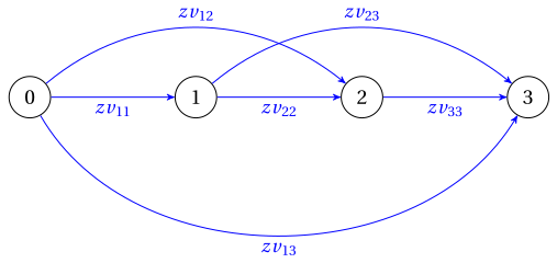
Network of the variables \(zv_{tk}\) for \(m=3\): the variable \(zv_{tk}\) is the arc from node \(t-1\) to node \(k\).
Example 15.4: \(\mathrm{MIP}^{\mathrm{SP}}_{\mathrm{CLSP}}\) model and combinations of paths
For the CLS instance of Example 15.1 the demands \(D_{t,k}\) and the costs \(cv_{tk}\) are (the production cost is zero, so \(cv_{tk}\) is only holding cost):
The \(\mathrm{MIP}^{\mathrm{SP}}_{\mathrm{CLSP}}\) model for this instance is:
An optimal solution \((\tilde{\vet{zv}},\tilde{\vet y})(\mathrm{MIP}^{\mathrm{SP}}_{\mathrm{CLSP}})\) is:
and all the other variables \(zv_{tk}\) are zero. It is the optimal plan \(\tilde{\vet x}=(3,0,4,4,0)\), which is not a path: in period \(3\) it produces \(4\) units, more than the demand \(3\) of period \(3\), and less than the demand \(7\) of the periods \(3\) and \(4\). It is the combination, with weights \(\tfrac{4}{5}\) and \(\tfrac{1}{5}\), of the paths \(0\to2\to3\to5\) (plan \((3,0,3,5,0)\)) and \(0\to2\to5\) (plan \((3,0,8,0,0)\)). The quantities are \(x_1=D_{1,2}\,zv_{12}=3\), \(x_3=3\cdot\tfrac{4}{5}+8\cdot\tfrac{1}{5}=4\) and \(x_4=5\cdot\tfrac{4}{5}=4\). The optimal value \(z(\mathrm{MIP}^{\mathrm{SP}}_{\mathrm{CLSP}})\) is
To obtain an LP relaxation of the \(\mathrm{MIP}^{\mathrm{SP}}_{\mathrm{CLSP}}\) model, we relax constraints \(\eqref{SP6}\) into the bounds \(0\le y_t\le 1\). The obtained LP model reads as follows:
This LP model is referred to as the \(\mathrm{LP}^{\mathrm{SP}}_{\mathrm{CLSP}}\) model.
Example 15.5: \(\mathrm{LP}^{\mathrm{SP}}_{\mathrm{CLSP}}\) model
The \(\mathrm{LP}^{\mathrm{SP}}_{\mathrm{CLSP}}\) model for the CLS instance of Example 15.1 is:
An optimal solution \((\tilde{\vet{zv}},\tilde{\vet y})(\mathrm{LP}^{\mathrm{SP}}_{\mathrm{CLSP}})\) is:
and all the other variables \(zv_{tk}\) are zero: the arcs of the optimal plan, with the setup of period \(4\) paid only for the fraction \(\tfrac{4}{5}\). The optimal value \(z(\mathrm{LP}^{\mathrm{SP}}_{\mathrm{CLSP}})\) is \(180-\tfrac{1}{5}\cdot 50=170\).
15.6 Comparing the formulations
-
The formulations have the same optimal value \(z(\mathrm{ILP}_{\mathrm{CLSP}})=z(\mathrm{MIP}^{\mathrm{SP}}_{\mathrm{CLSP}})=180\), but their LP relaxations have different optimal values. On the reference instance the lower bounds, computed with the exact simplex algorithm and checked with Gurobi, are the following.
-
The last column is the gap of Chapter 1 «Combinatorial optimization problems» between the bound and the optimal value; it is undefined for the bound \(0\).
| Model | Lower bound | Gap \(\frac{180-\LB}{\LB}\) |
|---|---|---|
| Without setups | \(0\) | undefined |
| \(\mathrm{LP}_{\mathrm{CLSP}}^{\mathrm{dem}}\) (\(M_t=D_{t,m}\)) | \(99.65\) | \(80.6\%\) |
| \(\mathrm{LP}_{\mathrm{CLSP}}^{\mathrm{cap}}\) (\(M_t=cap_t\)) | \(137.50\) | \(30.9\%\) |
| \(\mathrm{LP}_{\mathrm{CLSP}}^{\mathrm{strong}}\) (\(M_t=\min\{cap_t,D_{t,m}\}\)) | \(157.50\) | \(14.3\%\) |
| \(\mathrm{LP}_{\mathrm{CLSP}}^{\mathrm{SP}}\) (shortest path) | \(170\) | \(5.9\%\) |
-
The bound \(170\) of the shortest-path formulation is the optimal value of the problem without capacity (plan \((3,0,8,0,0)\), of cost \(170\)): the capacity constraints \(\eqref{LPSP4}\) act only on the quantities, and a combination of paths can satisfy them.
-
The price of the shortest-path formulation is its size: there are \(O(m^2)\) variables \(zv_{tk}\), against the \(O(m)\) variables of the big-M formulation.