6.2 The travelling salesman problem

Part 1 · Combinatorial optimization problems · Chapter 6 · Chapter 6: Routing problems · Lecture notes, volume 1 (PDF) · Slides · Exercises: Routing problems

Definition 6.1: Travelling salesman problem

Given:

1. a set \(\mathscr{V} = \{1,2,\dots,n\}\) of \(n\) cities,

2. for each pair of distinct cities \(i,j \in \mathscr{V}\), a distance \(d_{ij} \in \Z_{\ge 1}\), with \(d_{ij}=d_{ji}\),

the travelling salesman problem (TSP) asks to find a closed route that starts from a city, visits every other city exactly once and returns to the starting city, so that the total distance travelled is minimized.

• A TSP instance is specified by:

  1. one integer number:

     • the number of cities \(n \in \Z_{\ge 3}\),

  2. one symmetric matrix of integer numbers of size \(n \times n\):

     • \(D=(d_{ij})\), containing the distances; the diagonal entries are not used.

• A TSP feasible solution, called a tour, is a permutation of the cities

  \[ \sigma = (\sigma_1,\sigma_2,\dots,\sigma_n), \]

  read as the closed route \(\sigma_1 \to \sigma_2 \to \dots \to \sigma_n \to \sigma_1\). Its length is

  \[ L(\sigma) = \sum_{k=1}^{n-1} d_{\sigma_k \sigma_{k+1}} + d_{\sigma_n \sigma_1}, \]

  where the last term is the distance travelled to return to the starting city.

• Different permutations may describe the same tour: the starting city can be any of the \(n\) cities, and, since the distances are symmetric, the tour can be travelled in either direction.

  Given a TSP instance, the TSP can be formally stated as:

  \[\begin{equation*} \label{TSP} \tilde{\sigma} \in \argmin_{\sigma} \left\{ L(\sigma) = \sum_{k=1}^{n-1} d_{\sigma_k \sigma_{k+1}} + d_{\sigma_n \sigma_1} \;:\; \sigma \text{ is a permutation of } \mathscr{V} \right\}. \tag{6.1} \end{equation*}\]

• We denote by \(z(I)\) the length of an optimal tour \(\tilde{\sigma}\) of the instance \(I\).

6.2.1 Assumptions

• We make the following assumptions:

  1. There are at least three cities (with one or two cities there is only one route). Formally:

     \[ n \ge 3 \]

  2. The distances are symmetric (travelling from \(i\) to \(j\) costs as much as travelling from \(j\) to \(i\)). Formally:

     \[ d_{ij}=d_{ji},~~~~ \forall i,j \in \mathscr{V},~ i\neq j \]

Example 6.1: TSP instance

We consider a set \(\mathscr{V}=\{1,2,3,4,5\}\) of \(5\) cities (\(n=5\)), with the following distances:

\[ \begin{array}{c|ccccc} \hline {d_{ij}} & {1} & {2} & {3} & {4} & {5} \\ \hline {1} & --- & {5} & {2} & {2} & {9} \\ {2} & {5} & --- & {4} & {3} & {4} \\ {3} & {2} & {4} & --- & {4} & {7} \\ {4} & {2} & {3} & {4} & --- & {7} \\ {5} & {9} & {4} & {7} & {7} & --- \\ \hline \end{array} \]

The instance can be drawn as a complete graph, with one node per city and one edge, labelled with the distance, per pair of cities. The bold edges form the tour \(\sigma=(1,3,5,2,4)\), and the cities are drawn in the order of the tour:

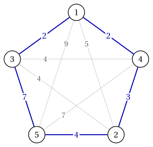
Its length is \(L(\sigma)=d_{13}+d_{35}+d_{52}+d_{24}+d_{41}=2+7+4+3+2=18\).

6.3 Counting the tours

Proposition 6.2

A TSP instance with \(n \ge 3\) cities has

\[ \frac{n!}{2n} = \frac{(n-1)!}{2} \]

distinct tours.

• There are \(n!\) permutations of the cities. Each tour is described by \(n\) permutations, one for every possible starting city, so there are \(n!/n=(n-1)!\) cyclic orderings of the cities.

• The distances are symmetric, so the tour travelled backwards has the same length and is not a new solution: every tour is counted twice, and we divide by \(2\).

Example 6.2: enumeration of the tours

The instance of Example 6.1 has \(\frac{(5-1)!}{2}=12\) distinct tours, which can be enumerated:

tour	\(L\)	tour	\(L\)	tour	\(L\)
\((1,3,5,2,4)\)	\(18\)	\((1,3,4,2,5)\)	\(22\)	\((1,2,3,5,4)\)	\(25\)
\((1,3,2,5,4)\)	\(19\)	\((1,4,3,2,5)\)	\(23\)	\((1,3,2,4,5)\)	\(25\)
\((1,2,5,3,4)\)	\(22\)	\((1,2,4,5,3)\)	\(24\)	\((1,4,2,3,5)\)	\(25\)
\((1,2,5,4,3)\)	\(22\)			\((1,2,4,3,5)\)	\(28\)
				\((1,2,3,4,5)\)	\(29\)

Hence the tour \(\sigma=(1,3,5,2,4)\) is the unique optimal tour, and \(z(I)=18\).

• The number of tours grows faster than any exponential function:

  \[ \begin{array}{rrrrr} \hline {n} & {5} & {10} & {15} & {20} \\ \hline {\frac{(n-1)!}{2}} & {12} & {181\,440} & {\approx 4.4\cdot 10^{10}} & {\approx 6.1\cdot 10^{16}} \\ \hline \end{array} \]

• A computer that evaluates \(10^9\) tours per second needs about \(6.1\cdot 10^{7}\) seconds, that is about two years, to list the tours of \(20\) cities. Enumeration is therefore useful only as a check on tiny instances, and the algorithms of this course must do better.

6.4 A first tour by hand

• The simplest way to build a tour is the nearest neighbour rule: start from a city and, as long as there are unvisited cities, move to the closest unvisited one; at the end, return to the starting city. In case of a tie we take the city with the smallest index.

Example 6.3: nearest neighbour from city \(1\)

On the instance of Example 6.1, starting from city \(1\):

1. from \(1\) the closest cities are \(3\) and \(4\), both at distance \(2\): we go to \(3\);

2. from \(3\) the unvisited cities \(2\) and \(4\) are both at distance \(4\): we go to \(2\);

3. from \(2\) the closest unvisited city is \(4\), at distance \(3\); then only \(5\) is left, at distance \(d_{45}=7\);

4. we return from \(5\) to \(1\) at distance \(d_{51}=9\).

The tour is \(\sigma=(1,3,2,4,5)\), of length \(2+4+3+7+9=25\).

• The last edges of the nearest neighbour tour are forced, and may be very long: here the final edge \(\{5,1\}\) costs \(9\). The tour of length \(25\) is worse than the optimal one, of length \(18\), by \(7\).

• From the nearest neighbour tour alone we cannot tell how far we are from the optimum: we need a lower bound.

6.5 A combinatorial lower bound

• For a city \(i\), let \(a_i \le b_i\) be the two smallest distances from \(i\) to the other cities.

Observation 6.3

For every symmetric TSP instance, the optimal length satisfies

\[ z(I) \;\ge\; \left\lceil \frac{1}{2} \sum_{i \in \mathscr{V}} (a_i + b_i) \right\rceil . \]

• In a tour, every city is entered by one edge and left by another one, so it has exactly two edges of the tour, each at least as long as \(a_i\) and \(b_i\) respectively.

• Summing over all the cities, every edge of the tour is counted twice, once for each of its end cities: hence \(2L(\sigma) \ge \sum_i (a_i + b_i)\) for every tour \(\sigma\).

• The distances are integer, so is \(L(\sigma)\), and we can round the bound up.

Example 6.4: the bound on the reference instance

For the instance of Example 6.1 the two smallest distances of each city are:

city \(i\)	\(1\)	\(2\)	\(3\)	\(4\)	\(5\)	sum
\(a_i\)	\(2\)	\(3\)	\(2\)	\(2\)	\(4\)
\(b_i\)	\(2\)	\(4\)	\(4\)	\(3\)	\(7\)
\(a_i+b_i\)	\(4\)	\(7\)	\(6\)	\(5\)	\(11\)	\(33\)

Hence \(z(I) \ge \lceil 33/2 \rceil = 17\). Together with the nearest neighbour tour we obtain

\[ 17 \le z(I) \le 25, \]

an absolute gap of \(8\), that is a relative gap of \(\frac{8}{17} \approx 47.1\%\). The tour \((1,3,5,2,4)\) of length \(18\) closes most of it, and only the enumeration of the \(12\) tours proves that \(18\) is optimal.

---

Next: 6.6 Variants: metric and asymmetric TSP