Approximation algorithms for the knapsack problem

Part 5 · Approximation algorithms · Chapter 35 · Lecture notes, volume 5 (PDF) · Slides (1/2) · Slides (2/2) · Exercises: 0/1 knapsack (KP) · App: 0/1 KP: greedy, Ext-Greedy, H² and FPTAS · App: Tight instances

Prerequisites

• From this module, the chapter «Principles of approximation algorithms»: performance ratio, relative and absolute performance guarantees, tightness, approximation schemes, PTAS and FPTAS.

• From this module, the chapters «Knapsack problems» and «Formulations of knapsack problems»: the KP, the LP relaxation \(\mathrm{LP}_{\mathrm{KP}}\) and the bound of Dantzig, which uses the split item.

• From this module, the chapters «Constructive heuristics» and «DP for the 0/1 knapsack problem»: the greedy algorithm and the dynamic programming by profits, used by the Basic-FPTAS algorithm.

Objectives

At the end of this chapter you will be able to:

• execute the greedy, Ext-Greedy, \(H^2\), \(H^{\ell}\) and Basic-FPTAS algorithms by hand on a KP instance;

• explain why the greedy algorithm has no constant guarantee, and why Ext-Greedy has guarantee \(2\);

• prove the guarantees \(\frac{4}{3}\) of \(H^2\), \(\frac{\ell+2}{\ell+1}\) of \(H^{\ell}\) and \(\frac{1}{1-\varepsilon}\) of the Basic-FPTAS algorithm;

• compare the running times of \(H^{\ell}\) and of the Basic-FPTAS algorithm, and say why only the second one is an FPTAS;

• explain why an absolute performance guarantee for the KP forces an exact algorithm.

The problem of this chapter is the 0/1 knapsack problem (KP): its definition and its assumptions are on its page.

35.1 Notation

• As on the problem page, \(c\) is the knapsack capacity and \(\mathscr{I}=\{1,2,\dots,n\}\) the set of items; in this chapter item \(i\in\mathscr{I}\) has profit \(p_i\) and weight \(w_i\).

• We denote by \(z(I)\) the optimal value of the KP on the instance \(I\), and by \(\mathscr{A}(I)\) the profit of the feasible solution returned by a heuristic algorithm \(\mathscr{A}\). Since every heuristic algorithm of this chapter returns a feasible solution,

  \[ \mathscr{A}(I) \le z(I) ~~~~~~~\text{and}~~~~~~~ \frac{z(I)}{\mathscr{A}(I)} \ge 1 \]

  for every KP instance \(I\).

• We assume throughout that the items are sorted by non-increasing efficiency

  \[ \frac{p_i}{w_i} \ge \frac{p_{i+1}}{w_{i+1}} \qquad \text{for all} \qquad i \in \{1,2,\dots,n-1\}, \]

  which requires \(O(n \log n)\) time, a polynomial function of the number \(n\) of items.

35.2 Split item and residual capacity

Definition 35.1: split item and residual capacity

Given a set \(\mathscr{I}=\{1,2,\dots,n\}\) of \(n\) items ordered by non-increasing efficiency, the split item is the item

\[\begin{equation*} {s} \in \mathscr{I} ~~~~\text{such that }~~~~ \sum_{i=1}^{s-1} w_i \leq c ~~~~\text{and }~~~~ \sum_{i=1}^{s} w_i > c \label{eq:split_item} \tag{35.1} \end{equation*}\]

and the residual capacity is

\[\begin{equation*} \mathit{rc} = c - \sum_{i=1}^{s-1} w_i \label{eq:residual_capacity} \tag{35.2} \end{equation*}\]

• The split item is the first one that does not fit entirely in the knapsack if all the previous ones are all selected.

• The residual capacity is the knapsack capacity remaining when all the items that precede the split item are selected.

• Sorting the items by non-increasing efficiency takes \(O(n \log n)\) time, and the split item is then found by scanning them. It is worth knowing that the split item can also be found in \(O(n)\) time, without sorting, by a weighted median search: the sorting is convenient, not necessary.

Example 35.1: split item and residual capacity

We consider a knapsack of capacity \(c = 9\) and a set \(\mathscr{I} = \{1,2,3,4,5,6,7\}\) of \(7\) items (\(n = 7\)), with the following profits and weights:

\[ \begin{array}{l|ccccccc} \hline & {i=1} & {i=2} & {i=3} & {i=4} & {i=5} & {i=6} & {i=7} \\ \hline {p_i} & {6} & {5} & {8} & {9} & {6} & {7} & {3} \\ {w_i} & {2} & {3} & {6} & {7} & {5} & {9} & {4} \\ \hline \end{array} \]

The efficiencies of the items are:

\[ \frac{p_1}{w_1}=\frac{6}{2},\quad \frac{p_2}{w_2}=\frac{5}{3},\quad \frac{p_3}{w_3}=\frac{8}{6},\quad \frac{p_4}{w_4}=\frac{9}{7},\quad \frac{p_5}{w_5}=\frac{6}{5},\quad \frac{p_6}{w_6}=\frac{7}{9},\quad \frac{p_7}{w_7}=\frac{3}{4}. \]

Thus the items are sorted by non-increasing efficiency: \((1,\,2,\,3,\,4,\,5,\,6,\,7)\). The split item is \(s=3\) since:

\[ \sum_{i=1}^{2} w_i = 2+3= 5 \le 9 \text{ and } \sum_{i=1}^{3} w_i = 2+3 + 6= 11 > 9 \]

and the residual capacity is:

\[ \mathit{rc} = c - \sum_{i=1}^{2} w_i = 9 - 2 - 3 = 4 \]

35.3 The greedy algorithm

• We assume items are sorted in non-increasing order of efficiency

  \[ \frac{p_i}{w_i} \ge \frac{p_{i+1}}{w_{i+1}} \quad \text{for all} \quad i \in \{1,2,\dots,n-1\} \]

The greedy algorithm (denoted by \(GR\)) is a constructive heuristic for the KP. It builds a feasible solution by processing the items in non-increasing order of efficiency, defined as the ratio between profit and weight. Starting from an empty subset of items, each item is added to the solution if and only if the capacity constraint is not violated.

• The pseudo-code of \(GR\) reads as follows:

Algorithm: Greedy

Input: KP instance \(I\) with \(n\) items, profits \(p[1..n]\), weights \(w[1..n]\), capacity \(c\)

Output: Feasible KP solution \(x[1..n]\)

1Function Greedy(\(n, p, w, c\))

2\(x := \text{new array}[1..n]\) ▹ selected items

3for \(i := 1\) to \(n\) do

4\(x[i] \leftarrow 0\) ▹ item \(i\) is initially not selected

5end

6\(rc := c\) ▹ residual capacity

7for \(i := 1\) to \(n\) do

8if \(w[i] \le rc\) then

9\(x[i] \leftarrow 1\) \(rc \leftarrow rc - w[i]\) ▹ select item \(i\) update residual capacity

10end

11end

12return \(x\)

Run in Colab:PythonC++

• Given the split item \(s\), \(GR\) selects all items that precede the split item, i.e.,

  \[ \{1,2,\dots,s-1\}\subseteq S \qquad\text{and}\qquad GR(I)\ge \sum_{i=1}^{s-1} p_i. \]

  Moreover, item \(s\) is not selected by \(GR\), while \(GR\) may also select some items that follow the split item.

Example 35.2: Execution of \(GR\)

For the KP instance of Example 35.1, the items are sorted by non-increasing efficiency:

\[ (1,\,2,\,3,\,4,\,5,\,6,\,7). \]

The execution of \(GR\) proceeds as follows:

1. Item \(1\) (weight \(w_1=2\)) is selected. The available capacity \(rc\) becomes \(9-2=7\).

2. Item \(2\) (weight \(w_2=3\)) is selected. The available capacity \(rc\) becomes \(7-3=4\).

3. Item \(3\) (weight \(w_3=6\)) is not selected since it does not fit into the available capacity \(rc=4\).

4. Item \(4\) (weight \(w_4=7\)) is not selected since it does not fit into the available capacity \(rc=4\).

5. Item \(5\) (weight \(w_5=5\)) is not selected since it does not fit into the available capacity \(rc=4\).

6. Item \(6\) (weight \(w_6=9\)) is not selected since it does not fit into the available capacity \(rc=4\).

7. Item \(7\) (weight \(w_7=4\)) is selected. The available capacity \(rc\) becomes \(4-4=0\).

Hence \(GR\) returns the feasible solution:

\[ S=\{1,2,7\}. \]

The total profit of the feasible solution is:

\[ GR(I)=\sum_{i\in S} p_i = p_1+p_2+p_7 = 6+5+3 = 14. \]

Therefore, \(14\) is a valid lower bound on the optimal value \(z(I)\):

\[ 14 \le z(I). \]

In this instance the split item is \(s=3\). Accordingly, \(GR\) selects all items preceding the split item, i.e., items \(1\) and \(2\), does not select item \(3\) (the split item), and then also selects item \(7\), which follows the split item.

Example 35.3: Execution of \(GR\)

We consider a knapsack of capacity \(c = 10\) and a set \(\mathscr{I} = \{1,2,3,4\}\) of \(4\) items (\(n = 4\)), with the following profits and weights:

\[ \begin{array}{l|cccc} \hline & {i=1} & {i=2} & {i=3} & {i=4} \\ \hline {p_i} & {6} & {8} & {19} & {4} \\ {w_i} & {2} & {3} & {9} & {5} \\ \hline \end{array} \]

The efficiencies of the items are:

\[ \frac{p_1}{w_1}=\frac{6}{2},\quad \frac{p_2}{w_2}=\frac{8}{3},\quad \frac{p_3}{w_3}=\frac{19}{9},\quad \frac{p_4}{w_4}=\frac{4}{5}. \]

Thus the items are sorted by non-increasing efficiency: \((1,\,2,\,3,\,4)\). The split item is \(s=3\) since:

\[ \sum_{i=1}^{2} w_i = 2+3= 5 \le 10 \ \ \text{ and }\ \ \sum_{i=1}^{3} w_i = 2+3+9= 14 > 10 \]

and the residual capacity is:

\[ \mathit{rc} = c - \sum_{i=1}^{2} w_i = 10 - 2 - 3 = 5. \]

The execution of \(GR\) proceeds as follows:

1. Item \(1\) (weight \(w_1=2\)) is selected. The available capacity \(rc\) becomes \(10-2=8\).

2. Item \(2\) (weight \(w_2=3\)) is selected. The available capacity \(rc\) becomes \(8-3=5\).

3. Item \(3\) (weight \(w_3=9\)) is not selected since it does not fit into the available capacity \(rc=5\).

4. Item \(4\) (weight \(w_4=5\)) is selected. The available capacity \(rc\) becomes \(5-5=0\).

Hence \(GR\) returns the feasible solution:

\[ S=\{1,2,4\}. \]

The total profit of the feasible solution is:

\[ GR(I)=\sum_{i\in S} p_i = p_1+p_2+p_4 = 6+8+4 = 18. \]

Therefore, \(18\) is a valid lower bound on the optimal value \(z(I)\):

\[ 18 \le z(I). \]

In this instance the split item is \(s=3\). Accordingly, \(GR\) selects all items preceding the split item, i.e., items \(1\) and \(2\), does not select item \(3\) (the split item), and then selects item \(4\), which follows the split item. Item \(3\) has the maximum profit (\(p_3=19\)) and it is optimal to select it alone, but it is not selected by \(GR\).

Example 35.4: Execution of \(GR\)

We consider a knapsack of capacity \(c = 10\) and a set \(\mathscr{I} = \{1,2,3,4,5\}\) of \(5\) items (\(n = 5\)), with the following profits and weights:

\[ \begin{array}{l|ccccc} \hline & {i=1} & {i=2} & {i=3} & {i=4} & {i=5} \\ \hline {p_i} & {4} & {6} & {5} & {12} & {3} \\ {w_i} & {1} & {2} & {2} & {6} & {2} \\ \hline \end{array} \]

The efficiencies of the items are:

\[ \frac{p_1}{w_1}=\frac{4}{1}=4,\quad \frac{p_2}{w_2}=\frac{6}{2}=3,\quad \frac{p_3}{w_3}=\frac{5}{2}=2.5,\quad \frac{p_4}{w_4}=\frac{12}{6}=2,\quad \frac{p_5}{w_5}=\frac{3}{2}=1.5. \]

Thus the items are sorted by non-increasing efficiency: \((1,\,2,\,3,\,4,\,5)\). The split item is \(s=4\) since:

\[ \sum_{i=1}^{3} w_i = 1+2+2= 5 \le 10 \ \ \text{ and }\ \ \sum_{i=1}^{4} w_i = 1+2+2+6= 11 > 10 \]

and the residual capacity is:

\[ \mathit{rc} = c - \sum_{i=1}^{3} w_i = 10 - 5 = 5. \]

The execution of \(GR\) proceeds as follows:

1. Item \(1\) (weight \(w_1=1\)) is selected. The available capacity \(rc\) becomes \(10-1=9\).

2. Item \(2\) (weight \(w_2=2\)) is selected. The available capacity \(rc\) becomes \(9-2=7\).

3. Item \(3\) (weight \(w_3=2\)) is selected. The available capacity \(rc\) becomes \(7-2=5\).

4. Item \(4\) (weight \(w_4=6\)) is not selected since it does not fit into the available capacity \(rc=5\).

5. Item \(5\) (weight \(w_5=2\)) is selected. The available capacity \(rc\) becomes \(5-2=3\).

Hence \(GR\) returns the feasible solution:

\[ S=\{1,2,3,5\}. \]

The total profit of the feasible solution is:

\[ GR(I)=\sum_{i\in S} p_i = p_1+p_2+p_3+p_5 = 4+6+5+3 = 18. \]

Therefore, \(18\) is a valid lower bound on the optimal value \(z(I)\):

\[ 18 \le z(I). \]

In this instance the split item is \(s=4\). Accordingly, \(GR\) selects items \(1\), \(2\), and \(3\) (which precede the split item), skips item \(4\) (the split item), and then selects item \(5\). The optimal solution is \(\tilde{S}=\{2,3,4\}\) with value \(z(I)=6+5+12=23\), which is better than the solution found by \(GR\).

Example 35.5: Execution of \(GR\)

We consider a knapsack of capacity \(c = 21\) and a set \(\mathscr{I} = \{1,2,3,4,5,6\}\) of \(6\) items (\(n = 6\)), with the following profits and weights:

\[ \begin{array}{l|cccccc} \hline & {i=1} & {i=2} & {i=3} & {i=4} & {i=5} & {i=6} \\ \hline {p_i} & {4} & {6} & {4} & {3} & {2} & {20} \\ {w_i} & {1} & {2} & {2} & {2} & {2} & {21} \\ \hline \end{array} \]

The efficiencies of the items are:

\[ \frac{p_1}{w_1}=\frac{4}{1}=4,\quad \frac{p_2}{w_2}=\frac{6}{2}=3,\quad \frac{p_3}{w_3}=\frac{4}{2}=2,\quad \frac{p_4}{w_4}=\frac{3}{2}=1.5,\quad \frac{p_5}{w_5}=\frac{2}{2}=1,\quad \frac{p_6}{w_6}=\frac{20}{21}. \]

Thus the items are sorted by non-increasing efficiency: \((1,\,2,\,3,\,4,\,5,\,6)\). The split item is \(s=6\) since:

\[ \sum_{i=1}^{5} w_i = 1+2+2+2+2= 9 \le 21 \ \ \text{ and }\ \ \sum_{i=1}^{6} w_i = 1+2+2+2+2+21= 30 > 21 \]

and the residual capacity is:

\[ \mathit{rc} = c - \sum_{i=1}^{5} w_i = 21 - 9 = 12. \]

The execution of \(GR\) proceeds as follows:

1. Item \(1\) (weight \(w_1=1\)) is selected. The available capacity \(rc\) becomes \(21-1=20\).

2. Item \(2\) (weight \(w_2=2\)) is selected. The available capacity \(rc\) becomes \(20-2=18\).

3. Item \(3\) (weight \(w_3=2\)) is selected. The available capacity \(rc\) becomes \(18-2=16\).

4. Item \(4\) (weight \(w_4=2\)) is selected. The available capacity \(rc\) becomes \(16-2=14\).

5. Item \(5\) (weight \(w_5=2\)) is selected. The available capacity \(rc\) becomes \(14-2=12\).

6. Item \(6\) (weight \(w_6=21\)) is not selected since it does not fit into the available capacity \(rc=12\).

Hence \(GR\) returns the feasible solution:

\[ S=\{1,2,3,4,5\}. \]

The total profit of the feasible solution is:

\[ GR(I)=\sum_{i\in S} p_i = p_1+p_2+p_3+p_4+p_5 = 4+6+4+3+2 = 19. \]

Therefore, \(19\) is a valid lower bound on the optimal value \(z(I)\):

\[ 19 \le z(I). \]

In this instance, the item with maximum profit is item \(6\) with \(p_6=20\), which appears last in the efficiency-sorted order. The greedy algorithm \(GR\) selects all items from \(1\) to \(5\) (which precede the split item), but does not select item \(6\) (the split item itself) because its weight \(w_6=21\) exceeds the residual capacity \(rc=12\). Item \(6\) alone would fit into the knapsack (since \(w_6=21 \le c=21\)) and would give a profit of \(20\), which is better than the greedy solution. The optimal solution is \(\tilde{S}=\{6\}\) with value \(z(I)=20\).

35.4 The Ext-Greedy algorithm

The Ext-Greedy algorithm (denoted by \(GR^e\)) is a constructive heuristic for the KP. It first computes a feasible solution by running the greedy algorithm \(GR\). Then it compares this solution with the best feasible solution consisting of a single item. Finally, it returns the better of the two solutions.

• The pseudo-code of \(GR^e\) reads as follows:

Algorithm: Extended Greedy

Input: KP instance \(I\) with \(n\) items, profits \(p[1..n]\), weights \(w[1..n]\), capacity \(c\)

Output: Feasible KP solution \(x[1..n]\)

1Function ExtendedGreedy(\(n, p, w, c\))

2\(x := Greedy(n, p, w, c)\) \(z := 0\) ▹ greedy solution value of the greedy solution

3for \(i := 1\) to \(n\) do

4if \(x[i] = 1\) then

5\(z \leftarrow z + p[i]\) ▹ add the profit of a selected item

6end

7end

8\(i_m := 1\) \(p_{\max} := p[1]\) ▹ best single item

9for \(i := 2\) to \(n\) do

10if \(p[i] > p_{\max}\) then

11\(i_m \leftarrow i\) \(p_{\max} \leftarrow p[i]\) ▹ update best single item update its profit

12end

13end

14\(\bar{x} := \text{new array}[1..n]\) ▹ best single-item solution

15for \(i := 1\) to \(n\) do

16\(\bar{x}[i] \leftarrow 0\)

17end

18\(\bar{x}[i_m] \leftarrow 1\) ▹ select only item \(i_m\)

19if \(z < p_{\max}\) then

20for \(i := 1\) to \(n\) do

21\(x[i] \leftarrow \bar{x}[i]\) ▹ copy component by component

22end

23end

24return \(x\)

Run in Colab:PythonC++

• Let \(p_{\max}\) be the maximum profit

  \[ p_{\max}=\max\big\{~p_i:\ i\in\mathscr{I} ~\big\}. \]

  and let \(\bar{S}\) be the best single-item feasible solution

  \[ \bar{S}=\big\{~i_m ~\big\} ~~\text{and}~~ i_m\in \arg\max\big\{~p_i:\ i\in\mathscr{I}~\big\} \]

Example 35.6: Execution of \(GR^e\)

We start from the feasible solution computed by \(GR\) on the KP instance of Example 35.1 (Example 35.2):

\[ S=\{1,2,7\}, \qquad GR(I)=\sum_{i\in S} p_i = p_1+p_2+p_7 = 6+5+3 = 14. \]

We now compute the maximum profit of a single item:

\[ p_{\max}=\max\big\{~p_i:\ i\in\mathscr{I} ~\big\}=p_4=9, \qquad \bar{S}=\{4\}. \]

Since \(14\ge 9\), \(GR^e\) keeps the greedy solution and returns

\[ S=\{1,2,7\}. \]

Example 35.7: Execution of \(GR^e\)

We start from the feasible solution computed by \(GR\) on the KP instance of Example 35.3:

\[ S=\{1,2,4\}, \qquad GR(I)=\sum_{i\in S} p_i = p_1+p_2+p_4 = 6+8+4 = 18. \]

We now compute the maximum profit of a single item:

\[ p_{\max}=\max\big\{~p_i:\ i\in\mathscr{I} ~\big\}=p_3=19, \qquad \bar{S}=\{3\}. \]

Since \(18<19\), \(GR^e\) replaces the greedy solution with the best single-item feasible solution and returns

\[ S=\{3\}. \]

• Given the split item \(s\), we have

  \[ GR^e(I)\ge GR(I)\ge \sum_{i=1}^{s-1} p_i. \]

  In addition, by definition of \(GR^e\), we have

  \[ GR^e(I)\ge p_{\max} \]

• For every KP instance \(I\), the objective values satisfy

  \[ GR(I)\ \le\ GR^e(I)\ \le\ z(I). \]

  This holds because \(GR^e\) returns the better between the greedy solution and the best single-item feasible solution, so it cannot be worse than \(GR\), and any feasible solution value is at most the optimal value \(z(I)\).

35.5 The \(H^2\) algorithm

The \(H^2\) algorithm is a constructive heuristic for the KP; it is the algorithm called \(G^{3/4}\) in the literature. It enumerates all feasible pairs of items \((i,k)\) and “guesses” that the two items belong to an optimal solution. For each pair, it fixes \(i\) and \(k\) in the knapsack, builds a residual instance using the remaining capacity and keeping only items with profit at most \(\min\{p_i,p_k\}\), and then completes the partial solution by running the Ext-Greedy algorithm \(GR^e\) on the residual instance. Finally, it returns the best solution found over all pairs, also comparing it with the best single-item feasible solution.

Algorithm: \(H^2\)

Input: KP instance \(I\) with item set \(\mathscr{I}=\{1,2,\dots,n\}\), profits \(p[1..n]\), weights \(w[1..n]\), capacity \(c\)

Output: Feasible KP value \(H^2(I)\)

1Function H2(\(\mathscr{I}, p, w, c\))

2\(p_{\max} := \max\{p[j]: j\in \mathscr{I}\}\)

3\(lb := p_{\max}\) \(\mathscr{P} := \big\{(i,k)\in \mathscr{I}\times\mathscr{I}: i<k,\ w[i]+w[k]\le c\big\}\) ▹ best value found

4for each \((i,k)\) in \(\mathscr{P}\) do

5\(\mathit{rc} := c-w[i]-w[k]\) \(\mathscr{I}(i,k) := \big\{j\in \mathscr{I}\setminus\{i,k\}: p[j]\le \min\{p[i],p[k]\},\ w[j]\le \mathit{rc}\big\}\) ▹ residual capacity

6\(I_{ik} := \text{KP instance restricted to } \mathscr{I}(i,k) \text{ with capacity } \mathit{rc}\)

7\(z_{res} := GR^e\big(I_{ik}\big)\) \(lb_{ik} := p[i]+p[k]+z_{res}\) ▹ value of \(GR^e\) on the residual instance

8if \(lb_{ik} > lb\) then

9\(lb \leftarrow lb_{ik}\)

10end

11end

12return \(lb\)

Run in Colab:PythonC++

Definition 35.2: feasible ordered pairs of items

Given a KP instance with item set \(\mathscr{I}=\{1,2,\dots,n\}\) and knapsack capacity \(c\), the set of all feasible ordered pairs of items is

\[\begin{equation*} \mathscr{P} = \Big\{~~ (i,k)\in \mathscr{I}\times\mathscr{I}:\ i<k,\ \ w_i+w_k\le c ~~\Big\}. \label{eq:feasible_pairs} \tag{35.3} \end{equation*}\]

• The \(H^2\) algorithm is based on the following idea: an optimal solution either consists of a single item, the one of maximum profit, or contains (at least) two items of “large” profit. The algorithm therefore guesses the two items of largest profit of an optimal solution, by enumerating all the feasible pairs in \(\mathscr{P}\), and completes each guess on a residual instance.

• The \(H^2\) algorithm considers the item pairs \((i,k) \in \mathscr{P}\), one at a time, and it executes three operations:

  1. The first operation consists of inserting items \(i\) and \(k\) into the knapsack. This creates a partial solution of profit \(p_i+p_k\) and a residual capacity \(c- w_i-w_k\).

  2. The second operation is the creation of a residual instance (denoted \(I(i,k)\)) containing only the items with profit smaller than or equal to the profits of the two inserted items. The residual set of item is:

     \[ \mathscr{I}(i,k)=\bigg\{j \in \mathscr{I} \setminus \{i,k\}:~~ p_j \le \min \big\{p_{i},p_{k}\},~~ w_{j} \le c - w_{i}-w_{k} \bigg\} \]

     The items with weight larger than the residual capacity are also discarded.

  3. The third operation is to complete the partial solution by executing the \(GR^e\) algorithm on the residual instance \(I(i,k)\).

• For each item pair \((i,k) \in \mathscr{P}\), we have the lower bound:

  \[ lb(i,k) = p_i+p_k + GR^e\big(I(i,k)\big) \]

  the global lower bound produced by the \(H^2\) algorithm is:

  \[ H^2(I) = \max \left\{ ~~\max_{(i,k) \in \mathscr{P}} \big\{ ~~lb(i,k)~~ \big\},~~ p_{\max} \right\} \]

This heuristic algorithm can be seen as “guessing” the two items with largest profit in an optimal solution (or the item with the largest profit).

Example 35.8: \(H^2\) algorithm

We consider a set \(\mathscr{I}=\{1,2,3,4,5,6,7\}\) of \(7\) items (\(n=7\)) with the following profits and weights:

item	\(p_j\)	\(w_j\)	\(\frac{p_j}{w_j}\)	efficiency
\(j=1\)	6	2	\(\frac{6}{2}\)	\(=3\)
\(j=2\)	5	3	\(\frac{5}{3}\)	\(\approx 1.66\)
\(j=3\)	8	6	\(\frac{8}{6}\)	\(\approx 1.33\)
\(j=4\)	9	7	\(\frac{9}{7}\)	\(\approx 1.28\)
\(j=5\)	6	5	\(\frac{6}{5}\)	\(=1.2\)
\(j=6\)	7	9	\(\frac{7}{9}\)	\(\approx 0.77\)
\(j=7\)	3	4	\(\frac{3}{4}\)	\(=0.75\)

and a knapsack capacity \(c=12\), so that \(p_{\max}=9\). The optimal solution is \(\tilde{S}=\{1,2,4\}\), of weight \(2+3+7=12\) and value \(z(I)=6+5+9=20\). The split item is \(s=4\), and \(GR^e\) returns the solution \(\{1,2,3\}\) with \(GR^e(I)=6+5+8=19\).

Execution of \(H^2\) (initialization \(lb=p_{\max}=9\)):

• Pair \((1,2)\): the residual capacity is \(\mathit{rc}=12-2-3=7\), \(\mathscr{I}(1,2)=\{7\}\) and \(GR^e\big(I(1,2)\big)=3\), hence \(lb(1,2)=6+5+3=14>lb\) and \(lb\) is updated to \(14\).

• Pair \((1,3)\): the residual capacity is \(\mathit{rc}=12-2-6=4\), \(\mathscr{I}(1,3)=\{2,7\}\) and \(GR^e\big(I(1,3)\big)=5\), hence \(lb(1,3)=6+8+5=19>lb\) and \(lb\) is updated to \(19\).

• Pair \((1,4)\): the residual capacity is \(\mathit{rc}=12-2-7=3\), \(\mathscr{I}(1,4)=\{2\}\) and \(GR^e\big(I(1,4)\big)=5\), hence \(lb(1,4)=6+9+5=20>lb\) and \(lb\) is updated to \(20\).

• Pair \((1,5)\): the residual capacity is \(\mathit{rc}=12-2-5=5\), \(\mathscr{I}(1,5)=\{2,7\}\) and \(GR^e\big(I(1,5)\big)=5\), hence \(lb(1,5)=6+6+5=17<lb\).

• Pair \((1,6)\): the residual capacity is \(\mathit{rc}=12-2-9=1\), \(\mathscr{I}(1,6)=\varnothing\), hence \(lb(1,6)=6+7=13<lb\).

• Pair \((1,7)\): the residual capacity is \(\mathit{rc}=12-2-4=6\), \(\mathscr{I}(1,7)=\varnothing\), hence \(lb(1,7)=6+3=9<lb\).

• The pairs \((i,k)\) with \(i \ge 2\) are processed in the same way, and none of them gives a value larger than \(20\). Hence \(H^2(I)=20=z(I)\): on this instance \(H^2\) finds the optimal solution, which \(GR^e\) misses.

Proposition 35.3

The \(H^2\) algorithm can be computed in \(O(n^3)\) time, and in \(O(n^2)\) time with a more careful implementation.

• We do not provide a formal proof but we only give the main ideas in what follows.

• The running time of the \(H^2\) algorithm is basically determined by executing the \(GR^e\) algorithm, which requires \(O(n)\) time, for every pair of items. This number of execution of \(GR^e\) is \(n \choose 2\) which is in \(O(n^2 )\) and hence the total running time is \(O(n^3)\).

• With a cleverer implementation it can be reduced to \(O(n^2 )\).

35.6 The \(H^{\ell}\) algorithm

The \(H^{\ell}\) algorithm is a constructive heuristic for the KP. It first computes the best feasible solution made of at most \(\ell-1\) items. Then it enumerates all the feasible sets \(L\) of exactly \(\ell\) items and “guesses” that they are the \(\ell\) items of largest profit of an optimal solution: for each set, it packs the items of \(L\), builds a residual instance with the remaining capacity and the items of profit at most \(\min\{p_i : i \in L\}\), and completes the partial solution by running the Ext-Greedy algorithm \(GR^e\) on the residual instance. Finally, it returns the best solution found.

Algorithm: \(H^{\ell}\)

Input: KP instance \(I\) with item set \(\mathscr{I}=\{1,2,\dots,n\}\), profits \(p[1..n]\), weights \(w[1..n]\), capacity \(c\), integer \(\ell\) with \(2\le\ell\le n\)

Output: Feasible KP value \(H^{\ell}(I)\)

1Function Hl(\(\mathscr{I}, p, w, c, \ell\))

2\(lb := \max\big\{\sum_{j\in S} p[j] : S \in \widehat{T}(\ell)\big\}\) ▹ feasible sets of at most \(\ell-1\) items

3for each \(L\) in \(T(\ell)\) do ▹ feasible sets of exactly \(\ell\) items

4\(\mathit{rc} := c-\sum_{i\in L} w[i]\) \(\mathscr{I}(L) := \big\{j\in \mathscr{I}\setminus L: p[j]\le \min_{i\in L} p[i],\ w[j]\le \mathit{rc}\big\}\) ▹ residual capacity

5\(lb_L := \sum_{i\in L} p[i] + GR^e\big(I(L)\big)\) ▹ complete the guess

6if \(lb_L > lb\) then

7\(lb \leftarrow lb_L\)

8end

9end

10return \(lb\)

Run in Colab:PythonC++

• The \(H^2\) algorithm guesses the two items of largest profit of an optimal solution. The \(H^{\ell}\) algorithm generalizes this idea: it guesses the \(\ell\) items of largest profit, for a fixed integer \(\ell\) with \(2 \le \ell \le n\). For \(\ell=2\) it is exactly the \(H^2\) algorithm.

• We define the collections of all feasible sets of exactly \(\ell\) items and of at most \(\ell-1\) items:

  \[ T(\ell) = \left\{ L \subseteq \mathscr{I}:~~ \sum_{j \in L} w_j \le c, ~~|L| = \ell \right\} \]

  and

  \[ {\widehat T}(\ell) = \left\{ L \subseteq \mathscr{I}:~~ \sum_{j \in L} w_j \le c, ~~|L| \le \ell-1 \right\} \]

• For each set \(L \in T(\ell)\) the algorithm executes three operations:

  1. it inserts all items \(i \in L\) into the knapsack, which creates a partial solution of profit \(\sum_{i \in L} p_i\) and a residual capacity \(c-\sum_{i \in L}w_i\);

  2. it creates the residual instance \(I(L)\), whose residual set of items is

     \[ \mathscr{I}(L)=\bigg\{j \in \mathscr{I} \setminus L:~~ p_j \le \min \big\{p_{i}: i \in L\},~~ w_{j} \le c - \sum_{i \in L} w_i \bigg\}; \]

  3. it completes the partial solution by running \(GR^e\) on \(I(L)\), which gives the value

     \[ lb(L) = \sum_{i \in L} p_i + GR^e\big(I(L)\big). \]

• The value returned by the algorithm is

  \[ H^{\ell}(I) = \max \left\{ \max_{L \in T(\ell)} lb(L),~~ \max_{S \in {\widehat T}(\ell)} \sum_{j \in S} p_j \right\}. \]

Example 35.9: Execution of \(H^{\ell}\)

We consider a knapsack of capacity \(c = 12\) and a set \(\mathscr{I} = \{1,2,3,4,5\}\) of \(5\) items (\(n=5\)), with the following profits and weights:

\[ \begin{array}{l|ccccc} \hline & {i=1} & {i=2} & {i=3} & {i=4} & {i=5} \\[1ex] \hline {p_i} & {2} & {3} & {3} & {3} & {3} \\[1ex] {w_i} & {1} & {3} & {3} & {3} & {3} \\[1ex] \hline \end{array} \]

The items are sorted by non-increasing efficiency, since \(\frac{2}{1}=2>\frac{3}{3}=1\). The optimal solution packs the four items of weight \(3\), with \(z(I)=12\).

With \(\ell=2\), i.e., the \(H^2\) algorithm of Section 35.5. A pair of two items of profit \(3\), for instance \(L=\{2,3\}\), leaves residual capacity \(6\) and the residual set \(\mathscr{I}(L)=\{1,4,5\}\): \(GR^e\) packs item \(1\) and item \(4\), of profit \(2+3=5\), so \(lb(L)=3+3+5=11\). A pair containing item \(1\) leaves an empty residual set, since no other item has profit at most \(2\). Hence \(H^2(I)=11<12\).

With \(\ell=3\). A set of three items of profit \(3\), for instance \(L=\{2,3,4\}\), leaves residual capacity \(3\) and the residual set \(\mathscr{I}(L)=\{1,5\}\): \(GR^e\) returns the best between item \(1\) alone (profit \(2\), then item \(5\) no longer fits) and item \(5\) alone (profit \(3\)), so \(lb(L)=9+3=12\). Hence \(H^3(I)=12=z(I)\).

Guessing one item more is enough to find the optimal solution on this instance, on which \(H^2\) does not.

Observation 35.4

The \(H^{\ell}\) algorithm can be computed in \(O(n^{\ell+1})\) time.

• The running time is determined by the executions of \(GR^e\), which requires \(O(n)\) time, one for every set in \(T(\ell)\). There are at most \(\binom{n}{\ell}\) such sets, which is in \(O(n^{\ell})\), hence the total running time is \(O(n^{\ell+1})\). With a more careful implementation it can be reduced to \(O(n^{\ell})\).

• Besides storing the input data, no significant additional memory is used, and the total space requirement is only \(O(n)\).

35.7 The Basic-FPTAS algorithm

• The \(H^{\ell}\) algorithm enumerates \(O(n^{\ell})\) sets of items, a number that grows very quickly with \(\ell\). The Basic-FPTAS algorithm follows a completely different route: instead of guessing items, it rounds the profits and solves the rounded instance exactly.

The Basic-FPTAS algorithm (denoted by \(FP^{\varepsilon}\)) replaces the item profits by scaled profits, which take few distinct values, and then solves the scaled instance to optimality by dynamic programming by profits. The optimal solution of the scaled instance is returned as a feasible solution of the original instance, which in general is not optimal.

Algorithm: Basic-FPTAS

Input: KP instance \(I\) with \(n\) items, profits \(p[1..n]\), weights \(w[1..n]\), capacity \(c\), accuracy \(\varepsilon \in (0,1)\)

Output: Feasible KP solution \(x[1..n]\)

1Function BasicFPTAS(\(n, p, w, c, \varepsilon\))

2\(lb := GR^e(I)\) \(K := \varepsilon \cdot lb / n\) ▹ value of the Ext-Greedy solution, a lower bound on \(z(I)\) scaling factor

3for \(j := 1\) to \(n\) do

4\(p'[j] \leftarrow \lfloor p[j]/K \rfloor\) ▹ scaled profit

5end

6\(Q := \lfloor 2n/\varepsilon \rfloor\) \(x := DPProfits(n, p', w, c, Q)\) ▹ upper bound on the optimal value of the scaled instance scaled instance solved to optimality, table truncated at \(Q\)

7return \(x\)

Run in Colab:PythonC++

• The scaling factor is

  \[ K = \frac{\varepsilon\,GR^e(I)}{n}, \]

  and the scaled profits are obtained by rounding down the profits to a multiple of \(K\):

  \[ p'_j = \left\lfloor \frac{p_j}{K} \right\rfloor \qquad \text{for all} \qquad j \in \mathscr{I}. \]

  The scaled instance \(I'\) has the same weights and the same capacity as \(I\), hence \(I\) and \(I'\) have exactly the same feasible solutions.

• The profits are scaled, not the weights. Rounding the weights down would make infeasible solutions look feasible, and rounding them up would discard solutions that are feasible: in both cases the scaled instance would answer a different question. Rounding the profits down, instead, keeps the set of feasible solutions untouched and only distorts the objective function.

• The scaled instance is solved by dynamic programming by profits, the second DP algorithm of the chapter «DP for the 0/1 knapsack problem»: \(u(j,q)\) is the minimum total weight of a subset of \(\{1,2,\dots,j\}\) of total profit exactly \(q\), and the optimal value is the largest \(q\) with \(u(n,q)\le c\).

• The table is truncated at \(Q=\lfloor 2n/\varepsilon\rfloor\). This is not smaller than the optimal value of the scaled instance, which is at most \(\frac{z(I)}{K}\le\frac{2\,GR^e(I)}{K}=\frac{2n}{\varepsilon}\) by the guarantee \(z(I)\le 2\,GR^e(I)\) of \(GR^e\). The table has size \(n\times Q\), and the running time is \(O(n\,Q)=O(n^2/\varepsilon)\).

Example 35.10: Execution of \(FP^{\varepsilon}\)

We consider a knapsack of capacity \(c = 8\) and a set \(\mathscr{I} = \{1,2,3,4\}\) of \(4\) items (\(n = 4\)), with the following profits and weights:

\[ \begin{array}{l|cccc} \hline & {i=1} & {i=2} & {i=3} & {i=4} \\[1ex] \hline {p_i} & {19} & {19} & {14} & {14} \\[1ex] {w_i} & {2} & {4} & {3} & {3} \\[1ex] \hline \end{array} \]

The items are sorted by non-increasing efficiency, since \(\frac{19}{2}=9.5 > \frac{19}{4}=4.75 > \frac{14}{3}\approx 4.67\). We run \(FP^{\varepsilon}\) with \(\varepsilon=\frac{1}{2}\).

Lower bound. \(GR\) packs item \(1\) (residual capacity \(8-2=6\)) and item \(2\) (residual capacity \(6-4=2\)), while items \(3\) and \(4\) do not fit, so \(GR(I)=19+19=38\). The best single item has profit \(19 \le 38\), hence

\[ GR^e(I)=38 . \]

Scaling. The scaling factor and the scaled profits are

\[ K = \frac{\varepsilon\,GR^e(I)}{n} = \frac{\frac{1}{2}\cdot 38}{4} = 4.75, \qquad p'_1=p'_2=\left\lfloor \frac{19}{4.75} \right\rfloor = 4, \qquad p'_3=p'_4=\left\lfloor \frac{14}{4.75} \right\rfloor = 2 . \]

The total scaled profit is \(P'=4+4+2+2=12\), not larger than \(Q=\lfloor 2n/\varepsilon\rfloor=16\), so the truncation does not act here.

Dynamic programming by profits. On the scaled instance, the minimum weights \(u(4,q)\) are

\[ \begin{array}{l|ccccccc} \hline {q} & {0} & {2} & {4} & {6} & {8} & {10} & {12} \\[1ex] \hline {u(4,q)} & {0} & {3} & {2} & {5} & {6} & {9} & {12} \\[1ex] \hline \end{array} \]

The largest \(q\) with \(u(4,q)\le c=8\) is \(q=8\), attained by the items \(\{1,2\}\) of total weight \(6\).

Solution returned. \(FP^{\varepsilon}\) returns \(S=\{1,2\}\), of true profit

\[ FP^{\varepsilon}(I)=19+19=38 . \]

The optimal solution is \(\tilde{S}=\{1,3,4\}\), of weight \(2+3+3=8\) and value \(z(I)=19+14+14=47\): the scaling has made items \(1\) and \(2\) look as good as items \(1\), \(3\) and \(4\) together. The performance ratio is

\[ \frac{z(I)}{FP^{\varepsilon}(I)}=\frac{47}{38}\approx 1.24 . \]

35.8 Performance guarantees

• We now determine the worst case performance ratio of the algorithms of the previous sections. Recall that, the KP being a maximization problem, the performance ratio of an algorithm \(\mathscr{A}\) on an instance \(I\) is \(z(I)/\mathscr{A}(I)\ge 1\), and that \(r(\mathscr{A})\) is its supremum over all the instances.

35.8.1 The worst case performance ratio of \(GR\)

Proposition 35.5

There are KP instances \(I\) such that:

\[\begin{equation*} \frac{ z(I) }{GR(I)} \to +\infty \qquad \text{as } c \to +\infty . \tag{35.4} \end{equation*}\]

Proof

Fix an integer \(\vartheta>2\) and consider the KP instance \(I_{\vartheta}\) with knapsack capacity \(c=\vartheta\) and the items set \(\mathscr{I}=\{1,2\}\), where the item profits and weights are

\[ p_1=2,\quad w_1=1, \qquad\text{and}\qquad p_2=\vartheta,\quad w_2=\vartheta. \]

An optimal solution packs item \(2\), and therefore

\[ z(I_\vartheta)=\vartheta. \]

Since

\[ \frac{p_1}{w_1}=2 \;>\; \frac{p_2}{w_2}=\frac{\vartheta}{\vartheta}=1, \]

\(GR\) packs item \(1\) first, leaving available capacity \(\vartheta-1\), so item \(2\) cannot be added. Thus

\[ GR(I_\vartheta)=2. \]

Hence,

\[ \lim_{\vartheta\to +\infty}\frac{z(I_\vartheta)}{GR(I_\vartheta)} = \lim_{\vartheta\to +\infty}\frac{\vartheta}{2} = +\infty. \]

□

• The proposition shows that there is no constant \(\alpha \in [1,+\infty)\) such that

  \[ \frac{z(I)}{GR(I)} \le \alpha \qquad \text{for all instances } I. \]

  Equivalently, the ratio \(\frac{z(I)}{GR(I)}\) can be made arbitrarily large by a suitable choice of the instance.

  In other words, there is no constant \(\alpha \in [1,+\infty)\) such that \(GR\) is an \(\alpha\)-approximation algorithm and the worst-case performance ratio of \(GR\) is unbounded:

  \[ r(GR)=+\infty. \]

• A key drawback of \(GR\) is that it may fail to select the item with maximum profit (even when that single item is optimal). In particular, by prioritizing efficiency \(p_i/w_i\), \(GR\) can fill the knapsack with high-efficiency items and leave insufficient available capacity to include the maximum-profit item.

35.8.2 The worst case performance ratio of \(GR^e\)

Proposition 35.6

For every KP instance \(I\), we have:

\[\begin{equation*} \frac{ z(I) }{GR^e(I)} \le 2 . \tag{35.5} \end{equation*}\]

Proof

Assume items are sorted by non-increasing efficiency. Let \(s\) be the split item and \(\mathit{rc}\) be the residual capacity. We have

\[ \underbrace{\sum_{i=1}^{s-1} p_i \;+\; p_s\frac{\mathit{rc}}{w_s}}_{=z\big({\rm LP_{KP}}\big)} \ \le\ \sum_{i=1}^{s-1} p_i \;+\; p_s \qquad\text{since}\qquad \mathit{rc} < w_s, \]

where \(z\big({\rm LP_{KP}}\big)\) is the optimal solution value of the LP relaxation of the natural ILP formulation of the KP. Accordingly,

\[ z(I) \le z\big({\rm LP_{KP}}\big) \le \sum_{i=1}^{s-1} p_i + p_s \le \sum_{i=1}^{s-1} p_i + p_{\max}, \]

since by definition of \(p_{\max}\) we have \(p_{\max}\ge p_s\).

Moreover,

\[ GR^e(I)\ge GR(I)\ge \sum_{i=1}^{s-1} p_i ~~~\text{and}~~~ GR^e(I)\ge p_{\max}. \]

Summing these two inequalities yields

\[ 2\,GR^e(I)=GR^e(I)+GR^e(I)\ \ge\ \sum_{i=1}^{s-1} p_i + p_{\max}. \]

Therefore,

\[ z(I)\le \sum_{i=1}^{s-1} p_i + p_{\max}\ \le\ 2\,GR^e(I). \]

Dividing by \(GR^e(I)>0\) yields

\[ \frac{z(I)}{GR^e(I)}\le 2. \]

□

Proposition 35.7

There are KP instances \(I\) such that:

\[\begin{equation*} \frac{ z(I) }{GR^e(I)} \to 2 \text{ as } c \to +\infty . \tag{35.6} \end{equation*}\]

Proof

Fix an integer \(\vartheta>2\) and consider the KP instance \(I_\vartheta\) with capacity \(c=2\vartheta\) and \(3\) items:

\[ p_1=2,\ w_1=1, \qquad p_2=\vartheta,\ w_2=\vartheta, \qquad p_3=\vartheta,\ w_3=\vartheta. \]

Items \(2\) and \(3\) fit together into the knapsack since \(w_2+w_3=2\vartheta=c\); hence an optimal solution packs items \(2\) and \(3\) and

\[ z(I_\vartheta)=2\vartheta. \]

Moreover,

\[ \frac{p_1}{w_1}=2 \;>\; \frac{p_2}{w_2}=\frac{p_3}{w_3}=1, \]

so \(GR\) packs item \(1\) first. After packing item \(1\), the available capacity is \(2\vartheta-1\), hence exactly one of items \(2\) and \(3\) can be added. Therefore \(GR\) returns a feasible solution of value \(\vartheta+2\). Since \(p_{\max}=\max\{p_1,p_2,p_3\}=\vartheta\), we have \(\vartheta+2>p_{\max}\), and thus

\[ GR^e(I_\vartheta)=\vartheta+2. \]

Consequently,

\[ \lim_{\vartheta\to +\infty}\frac{z(I_\vartheta)}{GR^e(I_\vartheta)} = \lim_{\vartheta\to +\infty}\frac{2\vartheta}{\vartheta+2} = \lim_{\vartheta\to +\infty}\frac{2}{1+\frac{2}{\vartheta}} = 2. \]

□

From Proposition 35.6 and Proposition 35.7 it follows that the worst case performance ratio of \(GR^e\) is two, i.e., we have

\[ r(GR^e)=2 \]

and \(GR^e\) is a \(2\)-approximation algorithm.

• A key strength of \(GR^e\) is that it mitigates the main weakness of \(GR\): even if the greedy packing misses a very profitable item because of the efficiency ordering, \(GR^e\) explicitly compares the greedy solution with the best single-item feasible solution and returns the better one, thereby guaranteeing a constant-factor approximation algorithm.

• However, the guarantee \(r(GR^e)=2\) is tight: there are instances in which \(GR^e\) is misled by efficiency and, after selecting an early high-efficiency item, it no longer has enough capacity to pack together the two items with the largest profits (which form the optimal solution), yielding a ratio arbitrarily close to \(2\).

• Getting a solution which is in the worst-case only half as good as the optimal solution does not sound very impressive.

• Hence, it is worthwhile trying to find a better approximation algorithm, possibly at the cost of an increased running time.

• In the previous worst-case example the \(GR^e\) made the “mistake” of excluding item \(3\) which had a very high profit value. To avoid such a mistake we need more advanced heuristic algorithms.

35.8.3 The worst case performance ratio of \(H^2\)

Proposition 35.8

For every KP instance \(I\), we have:

\[\begin{equation*} \frac{ z(I) }{H^2(I)} \le \frac{4}{3} . \tag{35.7} \end{equation*}\]

Proof

If \(z(I)\) is generated by a single item, we have \(H^2(I)=z(I)\).

Otherwise consider a feasible pair \((\tilde{\imath},\tilde{k}) \in \mathscr{P}\) which contributes the highest profit in an optimal solution. The residual instance is \(I(\tilde{\imath},\tilde{k})\) and the residual set of items is \(\mathscr{I}(\tilde{\imath},\tilde{k})\). The \(H^2\) algorithm considers this pair of items during its execution and applies \(GR^e\) on the residual instance \(I(\tilde{\imath},\tilde{k})\).

The pair contains the two items of largest profit of an optimal solution, so every other item of that solution has profit at most \(\min\{p_{\tilde{\imath}},p_{\tilde{k}}\}\) and fits into the residual capacity: it belongs to \(\mathscr{I}(\tilde{\imath},\tilde{k})\). The optimal solution value can therefore be written as:

\[\begin{equation*} z(I) = z\big(I(\tilde{\imath},\tilde{k})\big) + p_{\tilde{\imath}} + p_{\tilde{k}} \label{HHHH} \tag{35.8} \end{equation*}\]

where \(z\big(I(\tilde{\imath},\tilde{k})\big)\) is the optimal solution value of the residual instance \(I(\tilde{\imath},\tilde{k})\).

From of the operations of \(H^2\), we have:

\[\begin{equation*} H^2(I) ~~\ge~~ p_{\tilde{\imath}} + p_{\tilde{k}} + GR^e\big(I(\tilde{\imath},\tilde{k})\big) \label{KKKK} \tag{35.9} \end{equation*}\]

and since \(GR^e\) is a \(2\)-approximation algorithm, i.e., \(GR^e(I)\ge\frac{1}{2}\,z(I)\), we have:

\[ GR^e\big(I(\tilde{\imath},\tilde{k})\big) ~~\ge~~ \frac{1}{2} \: z\big(I(\tilde{\imath},\tilde{k})\big) \]

Accordingly:

\[ H^2(I) \ge p_{\tilde{\imath}} + p_{\tilde{k}} + \frac{1}{2} \: z\big(I(\tilde{\imath},\tilde{k})\big) \]

Moreover, due to \(\eqref{HHHH}\), we have:

\[ H^2(I) \ge p_{\tilde{\imath}} + p_{\tilde{k}} + \frac{1}{2} \big( z(I) - p_{\tilde{\imath}} - p_{\tilde{k}} \big) = \frac{1}{2} \big(z(I) + p_{\tilde{\imath}} +p_{\tilde{k}} \big) \]

We consider two possible cases:

• Case \(i)\):

  \[ p_{\tilde{\imath}} + p_{\tilde{k}} \ge \frac{1}{2}\: z(I) \]

  We have in this case:

  \[\begin{align*} H^2(I) & \ge \frac{1}{2} \big(z(I) + p_{\tilde{\imath}} +p_{\tilde{k}} \big)\\[2ex] &\ge \frac{1}{2} \left(z(I) + \frac{1}{2}\: z(I) \right) = \frac{3}{4} \: z(I) \end{align*}\]

  and accordingly

  \[ H^2(I) \ge \frac{3}{4} \: z(I) \]

• Case \(ii)\):

  \[ p_{\tilde{\imath}} + p_{\tilde{k}} < \frac{1}{2}\: z(I) \]

  Since their profits sum to less than \(\frac{1}{2}\,z(I)\), at least one of the two items \(\tilde{\imath}\), \(\tilde{k}\) has a profit smaller than \(\frac{1}{4}\,z(I)\).

  From LP\(_\text{KP}\) of the residual instance \(I(\tilde{\imath},\tilde{k})\), we have:

  \[\begin{align*} z\big(I(\tilde{\imath},\tilde{k})\big) &\le z\big({\rm LP_{KP}}\big)\\[2ex] &\le GR^e\big(I(\tilde{\imath},\tilde{k})\big)+ p_{s}\\[2ex] &\le GR^e\big(I(\tilde{\imath},\tilde{k})\big) + \frac{1}{4} \: z(I) \end{align*}\]

  where \(s\) is the split item of \(I(\tilde{\imath},\tilde{k})\) and \(p_s < \frac{1}{4} z(I)\) since all its items have a profit at most \(\min\{p_{\tilde{\imath}},p_{\tilde{k}}\}<\frac{1}{4} z(I)\) (by construction of the residual instance). If all the items of the residual instance fit into the residual capacity there is no split item: then \(GR^e\) packs all of them, \(z\big(I(\tilde{\imath},\tilde{k})\big)=GR^e\big(I(\tilde{\imath},\tilde{k})\big)\), and the inequalities hold with \(p_s:=0\).

  We have:

  \[\begin{align*} z(I) & = p_{\tilde{\imath}} + p_{\tilde{k}} + z\big(I(\tilde{\imath},\tilde{k})\big)\\[2ex] & \le \underbrace{p_{\tilde{\imath}} + p_{\tilde{k}} + GR^e\big(I(\tilde{\imath},\tilde{k})\big)}_{\le H^2(I), ~~ \text{eq. } \eqref{KKKK}} + \frac{1}{4} \: z(I) \\[2ex] & \le H^2(I) + \frac{1}{4} \: z(I) \end{align*}\]

  and accordingly:

  \[ H^2(I) \ge \frac{3}{4} \: z(I) \]

In both cases \(H^2(I) \ge \frac{3}{4}\,z(I)\), that is, dividing by \(H^2(I)>0\),

\[ \frac{z(I)}{H^2(I)} \le \frac{4}{3}. \]

□

Proposition 35.9

There are KP instances \(I_M\) such that:

\[\begin{equation*} \frac{ z(I_M) }{H^2(I_M)} \;\to\; \frac{4}{3} \qquad\text{as}\qquad M\to+\infty . \tag{35.10} \end{equation*}\]

Proof

Let us consider the KP instance \(I_M\) with capacity \(c=4\:M\) and \(5\) items:

\[ p_1=2,~~w_1= 1, \text{ and } p_2=p_3=p_4=p_5=M,~~w_2=w_3=w_4=w_5=M, \]

where \(M \in \Z_{\ge 1}, M>2\) is an integer number. An optimal solution packs the four big items, since \(w_2+w_3+w_4+w_5=4\:M=c\), hence

\[ z(I_M)=4\:M. \]

The efficiencies are

\[ \frac{p_1}{w_1}=2 ~~~~>~~~~ \frac{p_2}{w_2}=\frac{p_3}{w_3}=\frac{p_4}{w_4}=\frac{p_5}{w_5} = \frac{M}{M}=1 \]

so item \(1\) comes first in the efficiency order.

We consider the two possible kinds of pair examined by \(H^2\):

1. a pair of two big items: the residual capacity is \(2\:M\) and the residual instance keeps item \(1\) and the two remaining big items, so \(GR^e\) packs item \(1\) and one big item, for a total value of \(3\:M + 2\);

2. a pair consisting of item \(1\) and one big item: the residual instance is empty, because no item has profit at most \(\min\{2,M\}=2\), for a total value of \(M + 2\).

The first kind of pair gives the larger value, hence

\[ H^2(I_M)= 3\:M+2 \]

Consequently,

\[ \lim_{M\to\infty}\frac{z(I_M)}{H^2(I_M)} =\lim_{M\to\infty}\frac{4\:M}{3\:M+2} =\lim_{M\to\infty}\frac{4}{3+\frac{2}{M}} =\frac{4}{3}. \]

□

From Proposition 35.8 and Proposition 35.9 it follows that the worst case performance ratio of \(H^2\) is four thirds, i.e., we have

\[ r(H^2)=\frac{4}{3} \]

and \(H^2\) is a \(\frac{4}{3}\)-approximation algorithm. Guessing two items instead of one brings the ratio down from the \(2\) of \(GR^e\) to \(\frac{4}{3}\).

35.8.4 The worst case performance ratio of \(H^{\ell}\)

Proposition 35.10

For every KP instance \(I\), we have:

\[\begin{equation*} \frac{ z(I) }{H^{\ell}(I)} \le \frac{\ell+2}{\ell+1} . \tag{35.11} \end{equation*}\]

Proof

If an optimal solution contains at most \(\ell-1\) items, the algorithm finds it among the sets of \(\widehat{T}(\ell)\), and \(H^{\ell}(I)=z(I)\).

Otherwise, let \(\tilde{L} \in T(\ell)\) be the set of the \(\ell\) items of largest profit of an optimal solution. The algorithm considers \(\tilde{L}\) during its execution and applies \(GR^e\) to the residual instance \(I(\tilde{L})\). All the other items of the optimal solution belong to \(\mathscr{I}(\tilde{L})\), hence

\[\begin{equation*} z(I) = \sum_{i \in \tilde{L}} p_{i} + z\big(I(\tilde{L})\big), \label{eq:Hlsplit} \tag{35.12} \end{equation*}\]

where \(z\big(I(\tilde{L})\big)\) is the optimal value of the residual instance. From the operations of \(H^{\ell}\), and since \(GR^e\) is a \(2\)-approximation algorithm,

\[ H^{\ell}(I) \;\ge\; \sum_{i \in \tilde{L}} p_i + GR^e\big(I(\tilde{L})\big) \;\ge\; \sum_{i \in \tilde{L}} p_i + \frac{1}{2}\, z\big(I(\tilde{L})\big) \;=\; \frac{1}{2} \Big(z(I) + \sum_{i \in \tilde{L}} p_i \Big), \]

where the last equality follows from \(\eqref{eq:Hlsplit}\). We consider two cases.

• Case \(i)\): \(\displaystyle \sum_{i \in \tilde{L}} p_i \ge \frac{\ell}{\ell+2}\, z(I)\). Then

  \[ H^{\ell}(I) \;\ge\; \frac{1}{2} \left(z(I) + \frac{\ell}{\ell+2}\, z(I) \right) = \frac{\ell + 1 }{\ell + 2}\, z(I). \]

• Case \(ii)\): \(\displaystyle \sum_{i \in \tilde{L}} p_i < \frac{\ell}{\ell+2}\, z(I)\). Then at least one item of \(\tilde{L}\) has profit smaller than \(\frac{1}{\ell+2}\, z(I)\), and so do all the items of the residual instance, whose profits are at most \(\min\{p_i : i \in \tilde{L}\}\). Let \(s\) be the split item of \(I(\tilde{L})\) (if there is none, \(GR^e\) packs all the items of \(I(\tilde{L})\), and the inequalities below hold with \(p_s:=0\)). The LP relaxation of the residual instance gives

  \[ z\big(I(\tilde{L})\big) \;\le\; z\big({\rm LP_{KP}}\big) \;\le\; GR^e\big(I(\tilde{L})\big) + p_{s} \;<\; GR^e\big(I(\tilde{L})\big) + \frac{1}{\ell +2}\, z(I), \]

  and therefore, by \(\eqref{eq:Hlsplit}\),

  \[ z(I) \;<\; \sum_{i \in \tilde{L}} p_{i} + GR^e\big(I(\tilde{L})\big) + \frac{1}{\ell +2}\, z(I) \;\le\; H^{\ell}(I) + \frac{1}{\ell +2}\, z(I), \]

  that is, \(H^{\ell}(I) > \frac{\ell+1}{\ell+2}\, z(I)\).

In both cases \(H^{\ell}(I) \ge \frac{\ell+1}{\ell+2}\, z(I)\), and dividing by \(H^{\ell}(I)>0\) gives the statement. □

Proposition 35.11

There are KP instances \(I_M\) such that:

\[\begin{equation*} \frac{ z(I_M) }{H^{\ell}(I_M)} \;\to\; \frac{\ell+2}{\ell+1} \qquad\text{as}\qquad M\to+\infty . \tag{35.13} \end{equation*}\]

Proof

Fix an integer \(M>2\) and consider the KP instance \(I_M\) with capacity \(c=(\ell +2)\,M\) and \(n=\ell +3\) items, where

\[ p_1=2,~~w_1= 1, \text{ and } p_j=w_j=M ~~\text{for}~~ j \in \{2,3,\dots,n\}. \]

An optimal solution packs the \(\ell+2\) items of weight \(M\), which fill the knapsack, hence \(z(I_M)=(\ell +2)\,M\). Item \(1\) comes first in the efficiency order, since \(\frac{p_1}{w_1}=2>1\). The sets \(L\) examined by \(H^{\ell}\) are of two kinds:

1. \(L\) made of \(\ell\) items of profit \(M\): the residual capacity is \(2M\), the residual instance keeps item \(1\) and the two remaining items of profit \(M\), and \(GR^e\) packs item \(1\) and one of them, for a total value of \(\ell M + M + 2=(\ell+1)\,M + 2\);

2. \(L\) containing item \(1\) and \(\ell -1\) items of profit \(M\): the residual instance is empty, since no item has profit at most \(\min\{2,M\}=2\), for a total value of \((\ell -1)\,M + 2\).

The sets of at most \(\ell-1\) items give at most \((\ell-1)\,M+2\) as well. Hence \(H^{\ell}(I_M)= (\ell +1)\,M + 2\) and

\[ \lim_{M\to\infty}\frac{z(I_M)}{H^{\ell}(I_M)} =\lim_{M\to\infty}\frac{(\ell+2)\,M}{(\ell+1)\,M+2} =\lim_{M\to\infty}\frac{\ell+2}{\ell+1+\frac{2}{M}} =\frac{\ell+2}{\ell+1}. \]

For \(\ell=2\) this is the instance used for \(H^2\). □

From Proposition 35.10 and Proposition 35.11 it follows that the worst case performance ratio of \(H^{\ell}\) is

\[ r(H^{\ell})=\frac{\ell+2}{\ell+1} \]

and \(H^{\ell}\) is a \(\frac{\ell+2}{\ell+1}\)-approximation algorithm. For \(\ell=2\) we find again \(r(H^2)=\frac{4}{3}\), and the ratio tends to \(1\) as \(\ell\) grows.

35.8.5 Approximation schemes

• We recall the definitions of the chapter «Principles of approximation algorithms». The relative error of an algorithm \(\mathscr{A}\) on a KP instance \(I\) is \(\frac{z(I)-\mathscr{A}(I)}{z(I)}\). An approximation scheme is a family of algorithms \(\{\mathscr{A}_{\varepsilon}\}_{\varepsilon\in(0,1)}\) such that, for every \(\varepsilon\) and every instance \(I\), the relative error of \(\mathscr{A}_{\varepsilon}\) is at most \(\varepsilon\); for a maximization problem this means that \(\mathscr{A}_{\varepsilon}\) is a \(\frac{1}{1-\varepsilon}\)-approximation algorithm. The scheme is a PTAS if, for every fixed \(\varepsilon\), the running time of \(\mathscr{A}_{\varepsilon}\) is polynomial in the size of the instance, and an FPTAS if it is polynomial both in the size of the instance and in the accuracy \(\frac{1}{\varepsilon}\).

• By Proposition 35.10, \(H^{\ell}(I)\ge\frac{\ell+1}{\ell+2}\,z(I)\), hence the relative error of \(H^{\ell}\) is at most

  \[ 1-\frac{\ell+1}{\ell+2}=\frac{1}{\ell+2}, \]

  which tends to \(0\) as \(\ell\) grows:

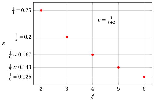
• The relation can be read the other way round: given the relative error \(\varepsilon\) to be attained, it is enough to choose \(\ell\) with \(\frac{1}{\ell+2}\le\varepsilon\), i.e., \(\ell \ge \frac{1}{\varepsilon}-2\).

By choosing

\[ \ell(\varepsilon) = \min \left\{ \max\left\{ \left\lceil \frac{1}{\varepsilon}\right\rceil -2,\; 2\right\},\; n \right\} \]

we obtain the \(H^{\varepsilon}\) algorithm, i.e., \(H^{\ell}\) with \(\ell=\ell(\varepsilon)\), whose relative error is at most \(\varepsilon\) for every \(\varepsilon \in (0,1)\).

• For \(\varepsilon \ge \frac{1}{4}\) we have \(\ell(\varepsilon)=2\), and \(H^{\varepsilon}\) is the \(H^2\) algorithm. The size \(\ell\) of the guessed sets cannot exceed \(n\), and with \(\ell=n\) the algorithm enumerates all the feasible solutions and is exact.

Observation 35.12

The family \(\{H^{\varepsilon}\}_{\varepsilon\in(0,1)}\) is a PTAS for the 0/1 knapsack problem.

• For every fixed \(\varepsilon\), \(\ell(\varepsilon)\) is a constant, and by Observation 35.4 the running time \(O\big(n^{\ell(\varepsilon)+1}\big)\) is polynomial in the size \(n\) of the instance.

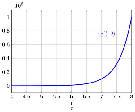
• However, \(H^{\varepsilon}\) is not an FPTAS: the exponent \(\ell(\varepsilon)=\left\lceil \frac{1}{\varepsilon}\right\rceil-2\) grows with the accuracy \(\frac{1}{\varepsilon}\), so the running time is not polynomial in \(\frac{1}{\varepsilon}\). The plot shows, for \(n=10\) items and \(4\le\frac{1}{\varepsilon}\le 8\), the number \(n^{\frac{1}{\varepsilon}-2}\), a lower bound on \(n^{\ell(\varepsilon)}\) (the cap \(\ell(\varepsilon)\le n\) is not active, since \(\frac{1}{\varepsilon}\le 12\)):

• The \(H^{\varepsilon}\) algorithm is a straightforward method and quite easy to implement, but its running time explodes as the required accuracy grows. Even for a moderate relative error \(\varepsilon=\frac{1}{10}\), i.e., a deviation of \(10\) percent from the optimal value, we have \(\ell(\varepsilon)=8\) and a running time of \(O(n^9)\), or still \(O(n^8)\) with the improved implementation.

35.8.6 The worst case performance ratio of the Basic-FPTAS

Proposition 35.13

For every KP instance \(I\) and every \(\varepsilon \in (0,1)\), we have:

\[\begin{equation*} \frac{ z(I) }{FP^{\varepsilon}(I)} \le \frac{1}{1-\varepsilon} . \tag{35.14} \end{equation*}\]

Proof

Let \(\tilde{S}\) be an optimal solution of \(I\) and let \(S\) be the solution returned by \(FP^{\varepsilon}\), i.e., an optimal solution of the scaled instance \(I'\). Since \(I\) and \(I'\) have the same feasible solutions, \(\tilde{S}\) is feasible for \(I'\) as well, and by optimality of \(S\) for \(I'\),

\[ \sum_{j\in S} p'_j \;\ge\; \sum_{j\in \tilde{S}} p'_j . \]

By definition of the scaled profits, \(K\,p'_j \le p_j\) and \(K\,p'_j > p_j-K\) for every item \(j\). Therefore

\[ FP^{\varepsilon}(I)=\sum_{j\in S} p_j \;\ge\; K\sum_{j\in S} p'_j \;\ge\; K\sum_{j\in \tilde{S}} p'_j \;>\; \sum_{j\in \tilde{S}} \big( p_j-K \big) \;=\; z(I) - |\tilde{S}|\,K . \]

Since an optimal solution contains at most \(n\) items and \(K = \varepsilon\,GR^e(I)/n\),

\[ |\tilde{S}|\,K \;\le\; n\,K \;=\; \varepsilon\,GR^e(I) \;\le\; \varepsilon\,z(I), \]

where the last inequality holds because \(GR^e(I)\) is the value of a feasible solution. Combining the two displays,

\[ FP^{\varepsilon}(I) \;\ge\; z(I) - \varepsilon\,z(I) \;=\; (1-\varepsilon)\,z(I), \]

and dividing by \(FP^{\varepsilon}(I)>0\) gives the statement. On the instance of Example 35.10, with \(\varepsilon=\frac{1}{2}\), the ratio is \(\frac{47}{38}\approx 1.24\), well below the bound \(\frac{1}{1-\varepsilon}=2\). □

Observation 35.14

The \(FP^{\varepsilon}\) algorithm can be computed in \(O\big(n^2/\varepsilon\big)\) time.

Proof

Let \(\tilde{q}\) be the optimal value of the scaled instance \(I'\). Every feasible solution of \(I'\) is feasible for \(I\), hence

\[ \tilde{q} \;\le\; \frac{z(I)}{K} \;\le\; \frac{2\,GR^e(I)}{K} \;=\; \frac{2\,GR^e(I)\,n}{\varepsilon\,GR^e(I)} \;=\; \frac{2n}{\varepsilon}, \]

where \(z(I)\le 2\,GR^e(I)\) is exactly the relative performance guarantee of \(GR^e\). Since \(\tilde{q}\) is an integer, \(\tilde{q}\le Q=\lfloor 2n/\varepsilon\rfloor\), and truncating the table of the dynamic program at \(Q\) does not change the result.

The table has \(n+1\) rows and \(Q+1\) columns, so the dynamic program runs in \(O(n\,Q)=O(n^2/\varepsilon)\) time, and the scaling and the call to \(GR^e\) take \(O(n)\) and \(O(n\log n)\) time.

Without the truncation, the table would reach the total scaled profit \(P'=\sum_{j}p'_j\). Since \(p_j\le GR^e(I)\) gives \(p'_j\le \frac{n}{\varepsilon}\), we only have \(P'\le \frac{n^2}{\varepsilon}\), which can be reached, and the running time would be \(O(n\,P')=O(n^3/\varepsilon)\). □

From Proposition 35.13 and Observation 35.14 it follows that the family \(\{FP^{\varepsilon}\}_{\varepsilon\in(0,1)}\) is an approximation scheme whose running time is polynomial both in the size \(n\) of the instance and in the accuracy \(\frac{1}{\varepsilon}\), i.e., an FPTAS for the 0/1 knapsack problem.

• The guarantee of \(GR^e\) is used twice, and in two different roles: \(GR^e(I)\le z(I)\) fixes the scaling factor, and \(z(I)\le 2\,GR^e(I)\) bounds the size of the dynamic programming table. A better heuristic in place of \(GR^e\) would shorten the table, not improve the guarantee.

35.9 Absolute performance guarantee

• Unfortunately, there is only a negative result concerning absolute performance guarantees for the 0/1 knapsack problem.

• The following theorem says that if an approximation algorithm would have an absolute performance guarantee \(k\) for some fixed \(k\), then this algorithm could be used to solve any instance of a 0/1 knapsack problem to optimality.

  Let \(f(n,c)\) be a function describing the running time of an algorithm for the KP with \(n\) items and capacity \(c\).

Theorem 35.15

Let \(\mathscr{A}\) be an approximation algorithm for the KP with absolute performance guarantee \(k\) and running time in \(O\big(f( n, c)\big)\) for any instance with \(n\) items and capacity \(c\). Then \(\mathscr{A}\) also computes the optimal solution of any such instance in \(O(f(n,c))\) time.

Proof

Consider an approximation algorithm \(\mathscr{A}\) for the KP with absolute performance guarantee \(k\) and let \(I\) be given by

\[ p_1,\dots,p_n,~~ w_1, \dots, w_n,~~c. \]

We construct the new instance \(I'\) with

\[ p'_1,\dots,p'_n,~~ w'_1, \dots, w'_n,~~c' \]

such that

\[ p'_j=(k+1)\:p_j,~~w_j'=w_j,~~\forall j \in \mathscr{I}, \text{ and } c'=c. \]

• Both instances \(I\) and \(I'\) have exactly the same set of feasible solutions.

• Since the objective function value of a solution of \(I'\) is exactly \(k + 1\) times as large as the objective function value of the same solution for \(I\), the two instances also have the same optimal solutions.

Applying algorithm \(\mathscr{A}\) to the instance \(I'\) yields a solution of value \(\mathscr{A}(I')\) with

\[ z(I')-\mathscr{A}(I') \le k \]

using the absolute performance guarantee of \(\mathscr{A}\).

Interpreting the output of \(\mathscr{A}\) as a solution for \(I\) yields a feasible solution of value \(\mathscr{A}(I)\), and

\[ \mathscr{A}(I') = (k+ 1) \: \mathscr{A}(I) \qquad\text{and}\qquad z(I')=(k+1)\,z(I) \]

Inserting in the above inequality yields

\[ (k+ 1)\: z(I) - (k+ 1)\: \mathscr{A}(I) \le k \Longleftrightarrow z(I) - \mathscr{A}(I) \le \frac{k}{k+1} \]

But since all profit values are integer, also \(z(I) - \mathscr{A}(I)\) must be integer and hence this inequality implies

\[ z(I) - \mathscr{A}(I) \le \left\lfloor \frac{k}{k+1} \right\rfloor \Longrightarrow z(I) - \mathscr{A}(I) \le 0 \Longrightarrow z(I) = \mathscr{A}(I) \]

Since the approximate solution of \(I'\) was computed in \(O(f(n,c))\) running time an optimal solution of \(I\) could be constructed within the same time. □

• This theorem indicates that an algorithm with fixed absolute performance guarantee for the KP would have the same unpleasant running time as an optimal algorithm.

  It is very unlikely that an exact algorithm for KP with a running time polynomial in \(n\) exists.

• Hence, also approximation algorithms with fixed absolute performance guarantee are bound to have a pseudo-polynomial running time which is unpleasantly dependent on the magnitude of the input values.

35.10 Typical mistakes

Warning

• Stopping the greedy algorithm at the split item. \(GR\) skips the split item \(s\) but keeps scanning, and it may select items that follow \(s\) (Example 35.2).

• Confusing \(i_m\) and \(s\). In \(GR^e\) the item \(i_m\) is the item of maximum profit \(p_{\max}\), not the split item \(s\): the two coincide only by chance.

• Forgetting to sort by efficiency. All the algorithms of this chapter assume the items sorted by non-increasing \(\frac{p_j}{w_j}\); the split item and the greedy solution depend on the order.

• Calling \(H^{\ell}\) an FPTAS. Its running time \(O(n^{\ell+1})\) has the exponent \(\ell(\varepsilon)=\lceil \frac{1}{\varepsilon}\rceil-2\) growing with \(\frac{1}{\varepsilon}\): \(H^{\varepsilon}\) is a PTAS, not an FPTAS.

• Scaling the weights. The Basic-FPTAS algorithm rounds down the profits only; the weights and the capacity are untouched, so that the feasible solutions are the same.

• Counting the whole table of the dynamic program. The bound \(O(n^2/\varepsilon)\) holds because the table is truncated at \(\lfloor 2n/\varepsilon\rfloor\); the total scaled profit can be as large as \(\frac{n^2}{\varepsilon}\).

35.11 In summary

In summary

• \(GR\) has no constant guarantee, \(GR^e\) (the better of \(GR\) and the best single item) has \(r(GR^e)=2\), \(H^2\) has \(r(H^2)=\frac{4}{3}\) and \(H^{\ell}\) has \(r(H^{\ell})=\frac{\ell+2}{\ell+1}\).

• \(\{H^{\varepsilon}\}\) is a PTAS with running time \(O(n^{\ell+1})\); the Basic-FPTAS algorithm rounds down the profits, solves the scaled instance exactly by dynamic programming, and is an FPTAS: it guarantees \(\frac{1}{1-\varepsilon}\) in time \(O(n^2/\varepsilon)\).

• No algorithm with a fixed absolute performance guarantee exists, unless it solves the KP exactly.

Dashboard of the KP instance of Example 35.1 (\(c=9\), \(p=(6,5,8,9,6,7,3)\), \(w=(2,3,6,7,5,9,4)\)). The bounds on \(z(I)\) found so far:

Source	Lower bound	Upper bound	From
Dantzig bound	–	\(16\)	\(\left\lfloor \frac{49}{3} \right\rfloor\), with \(s=3\) and \(rc=4\)
This chapter, \(GR\) and \(GR^e\)	\(14\)	–	\(S=\{1,2,7\}\)
This chapter, \(H^2\) and \(H^3\)	\(15\)	–	\(S=\{1,4\}\)
This chapter, \(FP^{\varepsilon}\) with \(\varepsilon=\frac{1}{2}\)	\(15\)	–	\(K=1\), the scaled instance is the original one
Best bounds	\(15\)	\(16\)	\(\UB-\LB=1\); the optimal value is \(15\)

---

Exercises on this chapter: 0/1 knapsack (KP)

In the interactive lab: 0/1 KP: greedy, Ext-Greedy, H² and FPTAS, Tight instances.