31.12 Multi-start local search
Part 4 · Heuristic algorithms · Chapter 31 · Chapter 31: Local search · Lecture notes, volume 4 (PDF) · Slides (1/2) · Slides (2/2) · Exercises: Local search · App: TSP: nearest neighbour and 2-opt
- Local search stops in the local optimum of the valley where it starts. The simplest way to explore other valleys is to start again from a different solution, and keep the best local optimum.
The multi-start local search (denoted by \(MSLS\)) generates \(M\) starting solutions, at random or with a randomized constructive heuristic, runs a local search from each of them, independently, and returns the best local optimum found.
Algorithm: Multi-start 2-opt
- The \(M\) local searches are independent: they can run in parallel, and the result does not depend on their order. Multi-start is the simplest form of diversification.
Example 31.11: \(MSLS\) on the TSP with \(10\) cities
On the instance of Example 31.3, \(100\) random tours (seed \(1\)), each improved by a local search, end in the following local optima:
| neighbourhood | rule | runs ending in the optimum \(39\) | other local optima (runs) |
|---|---|---|---|
| 2-opt | first | \(46\) | \(41\) (\(54\)) |
| 2-opt | best | \(87\) | \(41\) (\(8\)), \(43\) (\(5\)) |
| Or-opt | first | \(72\) | \(43\) (\(26\)), \(44\) (\(2\)) |
| Or-opt | best | \(77\) | \(43\) (\(22\)), \(44\) (\(1\)) |
| \(VND\) (2-opt, Or-opt) | first | \(100\) | — |
| \(VND\) (2-opt, Or-opt) | best | \(100\) | — |
With 2-opt and first improvement, the first random tour ends in the local optimum of length \(41\) and the third one in the optimum. On this instance, best improvement is much better than first improvement, and \(VND\) always finds the optimum, the only tour that is a local optimum for both neighbourhoods.
Example 31.12: \(MSLS\) on the TSP with \(30\) cities
The \(30\) cities have coordinates \((\lfloor 101u_{2k-1}\rfloor,\lfloor 101u_{2k}\rfloor)\), \(k=1,\dots,30\), where \(u_1,u_2,\dots\) are generated with seed \(12345\), and \(d_{ij}\) is the Euclidean distance rounded to the nearest integer. The optimal tour, computed with a MIP solver, has length \(z(I)=478\). The best of the \(30\) tours of \(NN\) (one for each starting city) has length \(537\).
The \(100\) random tours (seed \(1\)) have an average length of \(1768.73\) (between \(1364\) and \(2080\)). After the 2-opt local search:
| first improvement | best improvement | |
|---|---|---|
| distinct local optima | \(59\) | \(54\) |
| runs ending in the optimum | \(14\) | \(12\) |
| average length (relative error) | \(488.45\) (\(2.2\%\)) | \(487.24\) (\(1.9\%\)) |
| worst length (relative error) | \(537\) (\(12.3\%\)) | \(567\) (\(18.6\%\)) |
| first run that finds the optimum | \(2\) | \(9\) |
The local optima are distributed as follows (number of runs per class of length):
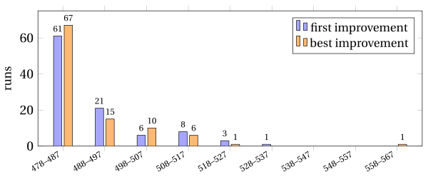
Local search turns tours of length about \(1769\) into tours within \(2\%\) of the optimum on average; but every run ends in its own valley, and only about one run in eight reaches the optimum.
31.12.1 The limits of multi-start
-
No memory. Each run starts from scratch and ignores what the previous runs found. If a run reaches the optimum with probability \(q\), independently of the others, \(M\) runs all miss it with probability \((1-q)^M\). With \(q=0.12\), as in the last example with best improvement, \(10\) runs miss the optimum with probability \(0.88^{10}\approx 0.28\), and \(37\) runs are needed to bring this probability below \(1\%\).
-
The probability \(q\) shrinks. The number of local optima grows very quickly with \(n\): on \(10\) cities only \(3\) tours are 2-opt local optima, on \(30\) cities \(100\) runs find more than \(50\) distinct ones. On large instances a random start almost never reaches the optimum, and \((1-q)^M\) is close to \(1\) for every reasonable \(M\).
-
Most of the time is spent descending. A random start is far from the good solutions, and the local search spends most of its moves on the descent from it; a good constructive heuristic gives better starting solutions, but few different ones.
-
A better strategy would use the local optima already found: restart near a good local optimum rather than anywhere, or continue the search from it by accepting some worse moves. These are the ideas of the metaheuristics.
31.12.2 What local search gives, and what it does not
-
Local search improves a feasible solution until it reaches a local optimum: a better primal bound, often much better than the starting one.
-
It does not give a dual bound, and the fact that it stopped does not mean that it arrived. On the \(30\)-city instance we know that \(478\) is optimal only because a MIP solver proved it; the local search alone could not tell the local optimum of length \(479\), found in many runs, from the optimum.
A local optimum is not a better bound: it is a feasible solution, i.e., one side of the gap. Its quality can be assessed only against a dual bound computed in another way.