32.9 Large neighbourhood search
Part 4 · Heuristic algorithms · Chapter 32 · Chapter 32: Metaheuristics · Lecture notes, volume 4 (PDF) · Slides (1/2) · Slides (2/2) · Exercises: Metaheuristics · App: TSP: simulated annealing and tabu search
Large neighbourhood search (denoted by \(LNS\)) improves a solution by destroying a part of it and repairing it: a destroy method removes some elements (items, cities, jobs) from the current solution, a repair method reinserts them, and the new solution replaces the current one if an acceptance criterion is satisfied. The neighbourhood of a solution is the set of all the solutions that destroy and repair can produce, and it is large.
- The pseudo-code of \(LNS\) for the TSP, which removes \(q\) random cities and reinserts them by cheapest insertion, reads as follows:
Algorithm: Large neighbourhood search for the TSP
-
\(LNS\) was introduced by Shaw (1998) for vehicle routing problems, where the repair was done by constraint programming. The size of the neighbourhood grows very quickly with the number \(q\) of removed elements: for the TSP there are \(\binom{n-1}{q}\) ways to choose the removed cities, and many ways to reinsert them. Such a neighbourhood cannot be listed and evaluated move by move, as in a local search: it is explored implicitly, by the repair method.
-
The repair method is a sub-algorithm: a constructive heuristic (cheapest insertion, FFD), or an exact algorithm for the subproblem left by the destroy method. The stronger the repair, the better the best neighbour found; the larger \(q\), the larger the neighbourhood, and the more expensive its exploration.
-
The destroy method diversifies (it is usually random, and \(q\) controls how far the search goes); the repair method intensifies (it rebuilds the destroyed part in the best way it can). Removing related elements (cities close to each other, items of the same bins) makes the repair more effective than removing unrelated ones, which can only be put back where they were.
Example 32.9: \(LNS\) on the TSP reference instance
From the nearest neighbour tour \((1,3,2,4,5)\) of length \(25\), with \(q=2\) and \(seed=1\). The first random number \(0.0000\) removes the city in position \(2+\lfloor 4\cdot 0.0000\rfloor=2\), city \(3\); the partial tour is \((1,2,4,5)\), and \(0.1315\) removes the city in position \(2+\lfloor 3\cdot 0.1315\rfloor=2\), city \(2\). The partial tour \((1,4,5)\) has length \(2+7+9=18\). Cheapest insertion of city \(3\):
so city \(3\) goes between \(5\) and \(1\): \((1,4,5,3)\). Cheapest insertion of city \(2\):
so city \(2\) goes between \(4\) and \(5\): \((1,4,2,5,3)\), of length \(18\), accepted. It is the optimal tour, traversed in the opposite direction: one destroy-and-repair step has changed four edges of the tour.
32.9.1 Large neighbourhood search for the BPP: heuristic and exact repair
-
For the BPP the natural destroy method empties bins: the least loaded bin, which is the one we would like to get rid of, and \(q-1\) other bins chosen at random. The repair method repacks the removed items into new bins, while the other bins are kept as they are. The new packing is accepted if it uses fewer bins, or the same number of bins and a value of the auxiliary objective \(\sum_b(\sum_{j\in P_b}w_j)^2\) not smaller: on the plateaus of the flat objective, the search moves toward fuller bins.
-
The repair solves a BPP subproblem, on the removed items only, and can do it in two ways: with FFD, or exactly, by a branch-and-bound that tries every bin for every item and keeps the packing with the fewest bins. The subproblem has only the items of \(q\) bins, so an exact repair is affordable.
Algorithm: Large neighbourhood search for the BPP
Example 32.10: \(LNS\) on the BPP reference instance
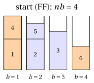
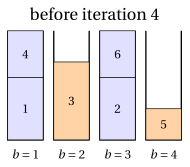
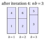
We start from the packing computed by First Fit, \(P_1=\{1,4\}\), \(P_2=\{2,5\}\), \(P_3=\{3\}\), \(P_4=\{6\}\), with loads \((7,6,5,3)\), and use \(q=2\), repair by FFD and \(seed=3\) (random numbers \(0.0000\), \(0.3946\), \(0.2668\), \(0.3760\)). At every iteration the least loaded bin is emptied, together with the bin in position \(1+\lfloor 3u\rfloor\) among the other three.
| it | loads | emptied | items | FFD | \(nb'\) | \(\sum_b(\cdot)^2\) |
|---|---|---|---|---|---|---|
| \(1\) | \((7,6,5,3)\) | \(P_4,P_1\) | \(\{1,4,6\}\) | \(\{1,4\}, \{6\}\) | \(4\) | \(119\to 119\) |
| \(2\) | \((6,5,7,3)\) | \(P_4,P_2\) | \(\{3,6\}\) | \(\{3\}, \{6\}\) | \(4\) | \(119\to 119\) |
| \(3\) | \((6,7,5,3)\) | \(P_4,P_1\) | \(\{2,5,6\}\) | \(\{2,6\}, \{5\}\) | \(4\) | \(119\to 127\) |
| \(4\) | \((7,5,7,2)\) | \(P_4,P_2\) | \(\{3,5\}\) | \(\{3,5\}\) | \(3\) | \(127\to 147\) |
Iterations \(1\) and \(2\) only reshuffle the items and keep the same loads (the auxiliary objective stays \(119\), and the new packing is accepted because it is not worse); iteration \(3\) builds the full bin \(\{2,6\}\), raising the auxiliary objective to \(127\); iteration \(4\) empties the bins \(\{5\}\) and \(\{3\}\), and FFD packs items \(3\) and \(5\) together: \(3\) bins, the optimum, and the search stops since \(nb=\LB\).
- On BPP24, starting from the FFD packing (\(10\) bins), with \(200\) iterations and \(seed=1,\dots,10\), the result depends on the repair:
| \(q\) | repair | bins at the end (10 seeds) | iterations to reach \(9\) |
|---|---|---|---|
| \(2\) | FFD | \(10,10,10,10,10,10,10,10,10,10\) | never |
| \(2\) | exact | \(10,10,10,10,10,10,10,10,10,10\) | never |
| \(3\) | FFD | \(10,10,10,10,10,10,10,10,10,10\) | never |
| \(3\) | exact | \(9,9,9,9,9,9,9,9,9,9\) | \(4,4,12,38,3,20,5,2,7,5\) |
| \(4\) | FFD | \(10,10,10,10,10,10,10,10,10,10\) | never |
| \(4\) | exact | \(9,9,9,9,9,9,9,9,9,9\) | \(2,3,9,12,4,5,1,3,10,2\) |
- With the FFD repair, \(LNS\) never improves the FFD packing: the items removed from an FFD packing are repacked by FFD in the same way. With the exact repair and \(q\ge 3\) it reaches the optimum in every run, in a few iterations: it finds three bins whose items fit into two, which is what FFD cannot see. With \(q=2\) even the exact repair fails, because the items of two bins of an FFD packing never fit into one.
A large neighbourhood is explored by solving a subproblem: the part of the solution left free by the destroy method is re-optimized, while the rest is fixed. The more powerful the method that solves the subproblem, the more powerful the neighbourhood.
32.9.2 Adaptive large neighbourhood search
- Which destroy method works best depends on the instance, and on the phase of the search. Adaptive LNS (ALNS), introduced by Ropke and Pisinger (2006), uses several destroy (and repair) methods, chooses one at random at every iteration, and learns which ones work, by giving to each method \(o\) a weight \(w_o\):
where \(\rho\in[0,1]\) is the reaction factor and the score \(\psi\) rewards the outcome of the iteration in which \(o\) was used: \(\psi=3\) if the new solution is the best found so far, \(2\) if it is better than the current one, \(1\) if it is as good, \(0\) if it is worse.
Algorithm: Adaptive large neighbourhood search for the TSP
-
WORSTREMOVAL removes, \(q\) times, the city whose removal shortens the tour the most: the city \(v\), between \(a\) and \(b\), of maximum \(d_{av}+d_{vb}-d_{ab}\). It is a deterministic, greedy destroy method: it removes the cities that seem badly placed.
-
On TSP20, from the nearest neighbour tour, with \(q=5\), \(200\) iterations and \(\rho=0.1\), ALNS reaches the optimum in \(7\) runs out of \(10\) (average \(299.4\)).
-
At the end the weight of the random removal is between \(0.77\) and \(0.98\), the weight of the worst removal between \(0.03\) and \(0.08\): the method has learnt that, from a good tour, removing the worst-placed cities and reinserting them by cheapest insertion almost always rebuilds a tour that is not better, and it has almost stopped using it.
-
In these runs plain \(LNS\) with random removal (\(q=5\)) does slightly better: adaptivity pays off when there are many methods, of unknown quality, and long runs.
Next: 32.10 Population-based methods: genetic and memetic algorithms