7.2 Scheduling on identical parallel machines

Part 1 · Combinatorial optimization problems · Chapter 7 · Chapter 7: Scheduling problems · Lecture notes, volume 1 (PDF) · Slides · Exercises: Scheduling problems

Definition 7.1: Scheduling on identical parallel machines

Given:

1. a set of \(m\) identical machines,

2. a set \(\mathscr{J} = \{1,2,\dots,n\}\) of \(n\) jobs,

3. for each job \(j \in \mathscr{J}\), a processing time \(t_j \in \Z_{\ge 1}\),

the problem \(P\,||\,C_{\max}\) asks to assign each job to a machine, so that the time needed to complete all the jobs, i.e., the largest total processing time assigned to a machine, is minimized.

• The name \(P\,||\,C_{\max}\) comes from the three-field notation of scheduling problems (Section 7.1.1).

• A \(P\,||\,C_{\max}\) instance is specified by:

  1. two integer numbers:

     • the number of machines \(m \in \Z_{\ge 1}\),

     • the number of jobs \(n \in \Z_{\ge 1}\),

  2. one vector of integer numbers of length \(n\):

     • \(\vet{t} \in \Z_{\ge 1}^n\), containing the processing times.

• A \(P\,||\,C_{\max}\) feasible solution is an assignment of the jobs to the machines, which we store in a vector \(\mathrm{mach}=(\mathrm{mach}_1,\mathrm{mach}_2,\dots,\mathrm{mach}_n)\):

  \[ \mathrm{mach}_j = h \quad \Longleftrightarrow \quad \text{job } j \text{ is assigned to machine } h . \]

  The set of jobs assigned to machine \(h\) is \(J_h = \{ j \in \mathscr{J} : \mathrm{mach}_j = h\}\), and its load is

  \[ L_h = \sum_{j \in J_h} t_j . \]

  Each machine processes its jobs one after the other, without idle times, so machine \(h\) completes its jobs at time \(L_h\). The makespan of the solution is the completion time of the last job,

  \[ C_{\max} = \max_{h \in \{1,2,\dots,m\}} L_h . \]

• The order in which a machine processes its jobs does not change its load: a solution is fully described by the sets \(J_1,J_2,\dots,J_m\), which form a partition of \(\mathscr{J}\) (some of them may be empty).

  Given a \(P\,||\,C_{\max}\) instance, the problem can be formally stated as:

  \[\begin{equation*} \label{PCmax} \min \left\{ \max_{h \in \{1,\dots,m\}} \sum_{j \in J_h} t_j \;:\; J_1,J_2,\dots,J_m \text{ is a partition of } \mathscr{J} \right\}. \tag{7.1} \end{equation*}\]

• We denote by \(z(I)\) the optimal makespan of the instance \(I\).

7.2.1 Assumptions

• We make the following assumption:

  1. There are more jobs than machines (otherwise each job gets a machine of its own, and the optimal makespan is \(\max_j t_j\)). Formally:

     \[ n > m \]

Example 7.1: \(P\,||\,C_{\max}\) instance

We consider \(m=3\) machines and a set \(\mathscr{J}=\{1,2,\dots,7\}\) of \(7\) jobs (\(n=7\)), with the following processing times:

\[ \begin{array}{l|ccccccc} \hline & {j=1} & {j=2} & {j=3} & {j=4} & {j=5} & {j=6} & {j=7} \\[1ex] \hline {t_j} & {5} & {5} & {4} & {4} & {3} & {3} & {3} \\ \hline \end{array} \]

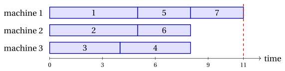
We call this instance Example 7.1: it is the reference instance of the chapter. The assignment \(\mathrm{mach}=(1,2,3,3,1,2,1)\) gives \(J_1=\{1,5,7\}\), \(J_2=\{2,6\}\), \(J_3=\{3,4\}\), with loads \(L_1=11\), \(L_2=8\), \(L_3=8\) and makespan \(11\):

7.3 Counting the solutions

• Every job can be assigned to any of the \(m\) machines, independently of the others: there are \(m^n\) assignments \(\mathrm{mach}\).

• The machines are identical, so two assignments that differ only by the names of the machines describe the same schedule. The distinct schedules are the partitions of \(\mathscr{J}\) into at most \(m\) non-empty sets, and their number is

  \[ \sum_{k=1}^{m} S(n,k), \]

  where \(S(n,k)\) is the Stirling number of the second kind, the number of partitions of \(n\) elements into exactly \(k\) non-empty sets.

Example 7.2: counting the schedules

For the instance of Example 7.1 there are \(3^7=2187\) assignments. The Stirling numbers are \(S(7,1)=1\), \(S(7,2)=63\) and \(S(7,3)=301\), so the distinct schedules are

\[ 1+63+301=365. \]

By enumeration, the schedules with the smallest makespan, \(9\), are exactly two:

\[ \{1,3\},\{2,4\},\{5,6,7\} \qquad \text{and} \qquad \{1,4\},\{2,3\},\{5,6,7\}, \]

which give \(3!\cdot 2=12\) of the \(2187\) assignments. The optimal schedule is therefore not unique.

• The growth is exponential in \(n\): with \(3\) machines, \(20\) jobs have \(3^{20} \approx 3.5\cdot 10^9\) assignments, and \(30\) jobs have \(3^{30} \approx 2.1\cdot 10^{14}\).

7.4 A first schedule by hand

• A simple way to build a schedule is to take the jobs one by one, in the order \(1,2,\dots,n\), and to assign each job to the machine with the smallest load at that moment; in case of a tie we take the machine with the smallest index.

Example 7.3: assigning every job to the least loaded machine

On the instance of Example 7.1 the loads of the three machines evolve as follows:

job \(j\) (\(t_j\))	machine chosen	loads \((L_1,L_2,L_3)\)
\(1\) (\(5\))	\(1\)	\((5,0,0)\)
\(2\) (\(5\))	\(2\)	\((5,5,0)\)
\(3\) (\(4\))	\(3\)	\((5,5,4)\)
\(4\) (\(4\))	\(3\)	\((5,5,8)\)
\(5\) (\(3\))	\(1\)	\((8,5,8)\)
\(6\) (\(3\))	\(2\)	\((8,8,8)\)
\(7\) (\(3\))	\(1\)	\((11,8,8)\)

We obtain the assignment \(\mathrm{mach}=(1,2,3,3,1,2,1)\) of the example, with makespan \(11\).

• When the last job arrives all the machines have load \(8\): whichever machine receives it, the largest load becomes \(8+3=11\).

• We do not know yet whether \(11\) is far from the optimal makespan: we need a lower bound.

7.5 A combinatorial lower bound

Observation 7.2

For every \(P\,||\,C_{\max}\) instance, the optimal makespan \(z(I)\) satisfies

\[ z(I) \;\ge\; \max\left\{ \max_{j\in\mathscr{J}} t_j,\;\; \left\lceil \frac{\sum_{j\in\mathscr{J}} t_j}{m} \right\rceil \right\}. \]

• The machine processing the longest job has load at least \(\max_j t_j\).

• The \(m\) loads sum up to \(\sum_j t_j\), so the largest one is at least their average \(\frac{1}{m}\sum_j t_j\), and, being an integer, at least its ceiling.

Example 7.4: the bound on the reference instance

On the instance of Example 7.1 the bound is \(\max\{5,\lceil 27/3\rceil\}=9\). Together with the schedule of Section 7.4,

\[ 9 \le z(I) \le 11. \]

The assignment \(\mathrm{mach}=(1,2,1,2,3,3,3)\) gives \(J_1=\{1,3\}\), \(J_2=\{2,4\}\), \(J_3=\{5,6,7\}\), all with load \(9\), and makespan \(9\):

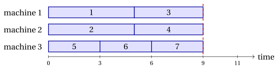
It attains the lower bound, so it is optimal: \(z(I)=9\). The three machines finish together, and no idle time is left before the makespan.

• The bound is not always attained. With \(m=2\) machines and three jobs of processing times \((4,3,3)\) it gives \(\max\{4,\lceil 10/2\rceil\}=5\), but the best schedule is \(\{1\},\{2,3\}\), with makespan \(6\).

7.6 Relation with the bin packing problem

• Given a value \(T\), a schedule with makespan at most \(T\) exists if and only if the jobs, seen as items of weight \(t_j\), can be packed into \(m\) bins of capacity \(T\): the machines are the bins and the loads are the total weights of the packing patterns.

• The two problems fix and minimize opposite quantities:

  	number of bins / machines	capacity / makespan
  BPP	minimized	fixed (\(c\))
  \(P\,||\,C_{\max}\)	fixed (\(m\))	minimized

• For this reason the two problems share many ideas: several heuristic algorithms for one of them have a counterpart for the other.

7.7 Remarks

• In 1966 R. L. Graham proved that any list of jobs, processed greedily, gives a makespan at most \(2-1/m\) times the optimal one.

• In 1969 he proved the better ratio \(4/3-1/(3m)\) for the list sorted by non-increasing processing time (the rule called LPT).

7.8 Typical mistakes

Warning

• Counting \(m^n\) different schedules. The machines are identical: renaming them gives the same schedule, so the distinct schedules are the partitions of the jobs into at most \(m\) sets.

• Confusing makespan and total load. The makespan is the largest load of a machine, not the sum of the processing times and not the average load.

• Forgetting the ceiling. The processing times are integer, so is the makespan: the average load \(27/3\) is rounded up when it is not an integer.

• Assuming that the bound is attained. The bound of Section 7.5 is a dual bound: a schedule with that makespan may not exist, as the instance \((4,3,3)\) on two machines shows.

• Believing that the optimal schedule is unique. The instance of Example 7.1 has two optimal schedules, and twelve optimal assignments.

7.9 In summary

In summary

• The problem \(P\,||\,C_{\max}\) asks to assign jobs to identical machines minimizing the largest load, the makespan; a solution is a partition of the jobs into at most \(m\) sets.

• There are \(m^n\) assignments, but only \(\sum_{k=1}^{m} S(n,k)\) distinct schedules.

• Giving each job to the least loaded machine builds a schedule quickly; the maximum between the longest job and the rounded average load is a lower bound on the optimal makespan.

• When a schedule attains the lower bound it is optimal; otherwise the gap remains open.

• The problem is the mirror of bin packing: here the number of machines is fixed and the capacity is minimized.

Dashboard of the \(P\,||\,C_{\max}\) instance (minimization: the lower bound is a dual bound, the upper bound is the makespan of a schedule):

Chapter	Lower bound	Upper bound	From
This chapter	\(9\)	\(11\)	longest job and average load; least loaded machine
This chapter, improved schedule	\(9\)	\(9\)	\(J_1=\{1,3\}\), \(J_2=\{2,4\}\), \(J_3=\{5,6,7\}\)

---

Exercises on this chapter: Scheduling problems

---

In depth: what the course does on this problem