31.8 \(P\,||\,C_{\max}\): move and swap
Part 4 · Heuristic algorithms · Chapter 31 · Chapter 31: Local search · Lecture notes, volume 4 (PDF) · Slides (1/2) · Slides (2/2) · Exercises: Local search · App: TSP: nearest neighbour and 2-opt
- The moves of \(P\,||\,C_{\max}\) transfer processing time between two machines: a move of job \(j\) from machine \(a\) to machine \(b\) transfers \(\delta=t_j\) from \(a\) to \(b\); a swap of jobs \(j\) (on \(a\)) and \(k\) (on \(b\)) transfers \(\delta=t_j-t_k\), which can be negative. In both cases the new loads are \(L_a-\delta\) and \(L_b+\delta\), and \(F(L,a,b,\delta)\) denotes the resulting change of the objective.
31.8.1 The move local search
The move local search for \(P\,||\,C_{\max}\) examines the reassignments of one job to another machine, applies an improving one chosen by the first- or the best-improvement rule, updates the two loads involved, and stops when no reassignment decreases the objective.
Algorithm: Move step for \(P\,||\,C_{\max}\)
31.8.2 The swap local search
The swap local search for \(P\,||\,C_{\max}\) examines the exchanges of two jobs on different machines, applies an improving one chosen by the first- or the best-improvement rule, updates the two loads involved, and stops when no exchange decreases the objective.
Algorithm: Swap step for \(P\,||\,C_{\max}\)
- For the makespan, the change of the objective is
computed in \(O(m)\) time from the loads \(L_1,\dots,L_m\) of the current solution.
-
A move or a swap is improving if and only if \(F(L,a,b,\delta)<0\). Since only \(L_a\) and \(L_b\) change, the makespan can decrease only if \(a\) is the unique critical machine: if another machine has load \(C_{\max}\), no move between two machines can lower the makespan.
-
An iteration costs \(O(nm^2)\) time for move and \(O(n^2m)\) for swap, because of the \(O(m)\) evaluation of \(F\); keeping the loads sorted reduces it, but the simple version is enough here.
-
A move changes the number of jobs on two machines, a swap keeps the number of jobs on every machine: if a machine has too many jobs, only a move can fix it, and the two neighbourhoods complement each other.
Example 31.5: The solution of \(LPT\) is a local optimum for move, but not for swap
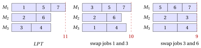
The solution of \(LPT\) on the \(P\,||\,C_{\max}\) reference instance has \(J_1=\{1,5,7\}\), \(J_2=\{2,6\}\), \(J_3=\{3,4\}\), loads \((11,8,8)\) and \(C_{\max}=11\). Machine \(1\) is the unique critical machine.
Move. The \(14\) moves give the loads
| move | loads | \(C_{\max}\) | move | loads | \(C_{\max}\) |
|---|---|---|---|---|---|
| job \(1\): \(M_1\to M_2\) | \((6,13,8)\) | \(13\) | job \(4\): \(M_3\to M_2\) | \((11,12,4)\) | \(12\) |
| job \(1\): \(M_1\to M_3\) | \((6,8,13)\) | \(13\) | job \(5\): \(M_1\to M_2\) | \((8,11,8)\) | \(11\) |
| job \(2\): \(M_2\to M_1\) | \((16,3,8)\) | \(16\) | job \(5\): \(M_1\to M_3\) | \((8,8,11)\) | \(11\) |
| job \(2\): \(M_2\to M_3\) | \((11,3,13)\) | \(13\) | job \(6\): \(M_2\to M_1\) | \((14,5,8)\) | \(14\) |
| job \(3\): \(M_3\to M_1\) | \((15,8,4)\) | \(15\) | job \(6\): \(M_2\to M_3\) | \((11,5,11)\) | \(11\) |
| job \(3\): \(M_3\to M_2\) | \((11,12,4)\) | \(12\) | job \(7\): \(M_1\to M_2\) | \((8,11,8)\) | \(11\) |
| job \(4\): \(M_3\to M_1\) | \((15,8,4)\) | \(15\) | job \(7\): \(M_1\to M_3\) | \((8,8,11)\) | \(11\) |
No move decreases the makespan: moving job \(1\) away from machine \(1\) makes the receiving machine reach \(8+5=13\), and moving job \(5\) or \(7\) lowers machine \(1\) to \(8\) but raises the receiving machine to \(8+3=11\). The solution of \(LPT\) is a local optimum for move, with \(C_{\max}=11\).
Swap. The first swap examined exchanges job \(1\) (on \(M_1\), \(t_1=5\)) and job \(3\) (on \(M_3\), \(t_3=4\)): \(\delta=1\), the loads become \((10,8,9)\) and \(C_{\max}=10\). It is improving, and first improvement accepts it at once; best improvement examines all the \(13\) swaps and finds two more with \(C_{\max}=10\) (jobs \(1\) and \(4\), jobs \(1\) and \(6\)), so it accepts the same swap, the first one found. Now \(J_1=\{3,5,7\}\), \(J_2=\{2,6\}\), \(J_3=\{1,4\}\).
In the second iteration, the swap of job \(3\) (on \(M_1\), \(t_3=4\)) and job \(6\) (on \(M_2\), \(t_6=3\)) has \(\delta=1\) and gives the loads \((9,9,9)\): it is found after \(9\) evaluations, and it is the only swap with \(C_{\max}<10\), so both rules accept it. The new solution \(J_1=\{5,6,7\}\), \(J_2=\{2,3\}\), \(J_3=\{1,4\}\) has \(C_{\max}=9=\left\lceil 27/3\right\rceil\): it is optimal.
-
On this example the move neighbourhood stops at \(11\), and the swap neighbourhood reaches the optimum \(9\). As observed for the KP in the chapter «Heuristic algorithms: definitions», the local optimum depends on the neighbourhood.
-
A larger neighbourhood does not always help. On the instance with \(m=4\) machines and \(12\) jobs with times \(t=(11,10,9,8,7,7,6,5,4,4,3,2)\), whose optimal makespan is \(z(I)=19=\lceil 76/4\rceil\), \(LPT\) gives \(J_1=\{1,8,10\}\), \(J_2=\{2,7,11\}\), \(J_3=\{3,6,12\}\), \(J_4=\{4,5,9\}\), with loads \((20,19,18,19)\): this solution is a local optimum for both move and swap.