3.6 Dijkstra's algorithm
Part 2 · Trees and paths · Chapter 3 · Chapter 3: Shortest paths · Lecture notes, volume 2 (PDF) · Exercises: Shortest paths · App: Shortest paths: Dijkstra, Bellman–Ford, acyclic graphs
- In this section all lengths are non-negative: \(d_{ij} \ge 0\) for every arc. Then every cycle has length \(\ge 0\), and (A2) holds.
- The nodes are permanent, when their label is final, or temporary. At every iteration the temporary node with the smallest label becomes permanent.
Algorithm: Dijkstra's algorithm
STOP.Theorem 3.22: correctness of Dijkstra's algorithm
If \(d_{ij} \ge 0\) for every arc, at every iteration of Dijkstra's algorithm:
-
(a) every permanent node \(i\) has \(d(i)=\tilde{d}(i)\);
-
(b) every temporary node \(j\) has as \(d(j)\) the minimum length of a path from \(s\) to \(j\) whose nodes other than \(j\) are all permanent (\(+\infty\) if there is none).
At the stop, \(d(j)=\tilde{d}(j)\) for every \(j \in N\).
Proof
Both properties hold after Step 0, with no permanent node. Let \(i\) be the node selected in Step 1.
-
\(d(i)=\tilde{d}(i)\). Let \(P\) be any path from \(s\) to \(i\), and let \(h\) be its first temporary node. The part of \(P\) up to \(h\) has length \(\ge d(h)\) by (b), and the rest has length \(\ge 0\), since \(d \ge 0\). Hence \(d(P) \ge d(h) \ge d(i)\), and by (b) the value \(d(i)\) is the length of a path: \(d(i)=\tilde{d}(i)\).
-
(b) after Step 2. Let \(j\) be temporary and \(Q\) a path to \(j\) whose other nodes are permanent, with \(h\) the node before \(j\). If \(h=i\), then \(d(Q) \ge \tilde{d}(i)+d_{ij}=d(i)+d_{ij}\), the value tested in Step 2.
-
If \(h \neq i\), then \(h\) became permanent before \(i\), through a path of permanent nodes of length \(\tilde{d}(h)\); when \(h\) was selected, Step 2 gave \(d(j) \le \tilde{d}(h)+d_{hj} \le d(Q)\).
Hence the new minimum is \(\min\{d(j),\,d(i)+d_{ij}\}\), attained by a path, which is the label left by Step 2. At the stop, the temporary nodes have \(d(j)=+\infty\): by (b) no arc leaves the permanent set towards them, so they are not reachable and \(\tilde{d}(j)=+\infty\). □
-
For the \(s\)–\(t\) problem the algorithm can stop as soon as \(t\) is permanent, by (a).
-
The arcs \((\mathit{pred}(j),j)\) form a shortest path tree: \(\mathit{pred}(j)\) is permanent before \(j\), and when it is last set \(d(j)=d(\mathit{pred}(j))+d_{\mathit{pred}(j)\,j}\) with both labels final.
Theorem 3.23: running time of Dijkstra's algorithm
With the labels in an array, Dijkstra's algorithm runs in \(O(n^2)\) time.
Proof
There are at most \(n\) iterations, and Step 1 scans the temporary labels in \(O(n)\) time. Step 2 scans the forward star of the selected node, and each node is selected once, so all the updates take \(O(m)\) time. The total is \(O(n^2+m)=O(n^2)\), since \(m \le n(n-1)\). □
- With the temporary labels in a binary heap, Step 1 and each decrease of a label take \(O(\log n)\) time: the total is \(O((n+m)\log n)\), better than \(O(n^2)\) on sparse graphs.
3.6.1 Dijkstra's algorithm on the reference graph
Example 3.9: Dijkstra from node \(1\)
We run the algorithm with the lengths of Example 3.1. Each row is an iteration: the selected node becomes permanent (bold label), and a label that decreased has the new predecessor in brackets.
| iteration | selected \(i\) | \(d(1)\) | \(d(2)\) | \(d(3)\) | \(d(4)\) | \(d(5)\) | \(d(6)\) |
|---|---|---|---|---|---|---|---|
| \(1\) | \(1\) | \(\mathbf{0}\) | \(7\) (\(1\)) | \(2\) (\(1\)) | \(\infty\) | \(\infty\) | \(\infty\) |
| \(2\) | \(3\) | \(\mathbf{0}\) | \(5\) (\(3\)) | \(\mathbf{2}\) | \(\infty\) | \(10\) (\(3\)) | \(\infty\) |
| \(3\) | \(2\) | \(\mathbf{0}\) | \(\mathbf{5}\) | \(\mathbf{2}\) | \(8\) (\(2\)) | \(10\) | \(\infty\) |
| \(4\) | \(4\) | \(\mathbf{0}\) | \(\mathbf{5}\) | \(\mathbf{2}\) | \(\mathbf{8}\) | \(10\) | \(13\) (\(4\)) |
| \(5\) | \(5\) | \(\mathbf{0}\) | \(\mathbf{5}\) | \(\mathbf{2}\) | \(\mathbf{8}\) | \(\mathbf{10}\) | \(13\) |
| \(6\) | \(6\) | \(\mathbf{0}\) | \(\mathbf{5}\) | \(\mathbf{2}\) | \(\mathbf{8}\) | \(\mathbf{10}\) | \(\mathbf{13}\) |
-
In iteration \(2\) the label of node \(2\) drops from \(7\) to \(2+3=5\); in iteration \(5\) the arc \((5,6)\) offers \(10+7=17>13\), and the arc \((5,4)\) ends in a permanent node.
-
The nodes become permanent in the order \(1,3,2,4,5,6\), with \(\tilde{d}=(0,5,2,8,10,13)\); the predecessors give the shortest path tree of Example 3.3.
3.6.2 Negative lengths
Example 3.10: a negative arc breaks Dijkstra's algorithm
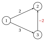
In the graph below, with \(s=1\), the algorithm makes node \(2\) permanent with \(d(2)=2\), then node \(3\) with \(d(3)=3\); the arc \((3,2)\) ends in a permanent node and is ignored. The path \(1,3,2\) has length \(3-2=1<2\).
On the reference graph with the lengths \(d'\) of Example 3.7 (\(d'_{54}=-3\)), Dijkstra's algorithm makes the nodes permanent in the order \(1,3,2,4,5,6\) and returns \(d(4)=8\) and \(d(6)=13\): node \(4\) is permanent before node \(5\), so the shorter path \(1,3,5,4\) of length \(7\) is missed, and with it the path to \(6\) of length \(12\).
- The proof of Theorem 3.22 uses \(d \ge 0\) in one point: the rest of \(P\) after its first temporary node has length \(\ge 0\). A negative arc breaks exactly this step.
With non-negative lengths, Dijkstra's algorithm makes permanent, at every iteration, the temporary node with the smallest label, whose label is then final; it runs in \(O(n^2)\) time. With a negative arc it can fail, and the Bellman–Ford algorithm is used instead.
3.7 Typical mistakes
Warning
-
Running Dijkstra's algorithm with a negative arc. Its labels can be wrong, as with \(d'_{54}=-3\) on the reference graph; use Bellman–Ford, or the topological order if the graph is acyclic.
-
Adding a constant to every length. It makes the lengths non-negative but changes the shortest paths: a path with \(k\) arcs grows by \(k\) times the constant.
-
Swapping the sign of the potentials. With \(+1\) in the tail of \(\mat{B}\) the dual constraints are \(\pi_i-\pi_j \le d_{ij}\) and the optimal potentials are \(\pi_i=-\tilde{d}(i)\).
-
Skipping the test of pass \(n\). After \(n-1\) passes the labels are the distances only without negative cycles; a change in pass \(n\) reveals one.
-
Expecting Bellman–Ford to see every negative cycle. It detects only the cycles reachable from \(s\), while a negative cycle anywhere in \(G\) makes the LP model unbounded.
-
Updating a permanent node in Dijkstra's algorithm. Its label is final; only temporary nodes are updated.
-
Looking for a topological order in a graph with cycles. It exists only in acyclic graphs: the reference graph has none.
3.8 In summary
In summary
-
The distance \(\tilde{d}(j)\) is the length of a shortest path from \(s\) to \(j\); it is well defined when no negative cycle is reachable from \(s\) (A2).
-
Subpaths of shortest paths are shortest; the distances satisfy Bellman's equations, and a shortest path tree exists.
-
Feasible potentials, \(\bar{c}_{ij}=d_{ij}-\pi_i+\pi_j \ge 0\), and a path of tight arcs certify optimality.
-
The LP model is a unit flow, \(\mat{B}\vet{x}=\vet{b}\), \(\vet{x} \ge \vet{0}\); its dual is \(\max\{\pi_s-\pi_t : \pi_i-\pi_j \le d_{ij}\}\), optimal at \(\pi_i=-\tilde{d}(i)\).
-
Acyclic graphs: topological order, \(O(n+m)\), any lengths. Bellman–Ford: \(O(n\,m)\), any lengths, detects negative cycles. Dijkstra: \(O(n^2)\), non-negative lengths.
The reference graph at a glance.
| lengths \(d\) (Dijkstra) | \(\tilde{d}=(0,5,2,8,10,13)\), order \(1,3,2,4,5,6\) |
| LP models | \(z(\mathrm{SP}(1,6))=13\), \(z(\mathrm{SP}(1))=38\) |
| lengths \(d'\), \(d'_{54}=-3\) (Bellman–Ford) | \(\tilde{d}=(0,5,2,7,10,12)\), \(5\) passes |
| lengths \(d''\), \(d''_{54}=-10\) | negative cycle \(3,5,4,3\) of length \(-1\) |
| acyclic graph, arc \((3,4)\) | order \(1,3,2,5,4,6\); \(\tilde{d}=(0,5,2,3,10,8)\) |
Exercises on this chapter: Shortest paths