6.5 A first feasible flow
Part 3 · Flows · Chapter 6 · Chapter 6: Minimum cost flow · Lecture notes, volume 3 (PDF) · Exercises: Minimum cost flow
- An algorithm that improves a feasible flow needs a feasible flow to start from. By the substitution of Chapter 4 we can assume \(\vet{l}=\vet{0}\).
Definition 6.11: auxiliary network
Let \(G=(N,A)\) be a balanced network with \(\vet{l}=\vet{0}\), and \(D=\sum_{i \in N: b_i>0} b_i\) its total supply. The auxiliary network adds to \(G\) a super source \(s\) and a super sink \(t\), an arc \((s,i)\) with capacity \(b_i\) for every supply node \(i\), and an arc \((i,t)\) with capacity \(-b_i\) for every demand node \(i\); the arcs of \(A\) keep their capacities.
Proposition 6.12: a feasible flow from a maximum flow
The network \(G\) has a feasible flow if and only if the maximum \(s\)–\(t\) flow of the auxiliary network has value \(D\). In that case, a maximum flow restricted to the arcs of \(A\) is a feasible flow of \(G\).
Proof
The value of an \(s\)–\(t\) flow is the flow leaving \(s\), at most the total capacity \(D\) of the arcs \((s,i)\).
-
Only if. Let \(\vet{x}\) be feasible, and set \(x_{si}=b_i\) on the arcs \((s,i)\) and \(x_{it}=-b_i\) on the arcs \((i,t)\). At a supply node the outflow minus inflow becomes \(b_i-x_{si}=0\), at a demand node \(b_i+x_{it}=0\), and transshipment nodes do not change: this is an \(s\)–\(t\) flow of value \(D\), hence maximum.
-
If. Let a maximum flow have value \(D\). Then all the arcs \((s,i)\) are saturated. The value is also the flow entering \(t\), and the arcs \((i,t)\) have total capacity \(\sum_{i: b_i<0}(-b_i)=D\), since the network is balanced: they are saturated too.
-
Conservation at \(i \in N\) then gives, along the arcs of \(A\), outflow minus inflow equal to \(x_{si}-x_{it}=b_i\), and the capacities hold: the restriction to \(A\) is a feasible flow. □
-
We compute the maximum flow with the Edmonds–Karp algorithm of Chapter 5: a breadth-first search from \(s\) in the residual network, scanning the arcs that leave a node by increasing index of the head (\(s\) before node \(1\), \(t\) after node \(n\)).
-
The maximum flow ignores the costs: it gives a feasible flow, usually far from optimal.
Example 6.5: a feasible flow of the reference network
The reference network has \(D=5+2=7\). The auxiliary network adds the arcs \((s,1)\), \((s,2)\) with capacities \(5\), \(2\), and \((4,t)\), \((6,t)\) with capacities \(3\), \(4\) (red and dashed in the figure). The augmenting paths of the Edmonds–Karp algorithm are:
| path | nodes | units |
|---|---|---|
| \(1\) | \(s,2,4,t\) | \(2\) |
| \(2\) | \(s,1,2,4,t\) | \(1\) |
| \(3\) | \(s,1,2,4,6,t\) | \(1\) |
| \(4\) | \(s,1,3,5,6,t\) | \(2\) |
| \(5\) | \(s,1,3,5,4,6,t\) | \(1\) |
The value is \(7=D\), so the network has a feasible flow. Each arc carries \(x_{ij}/u_{ij}\):
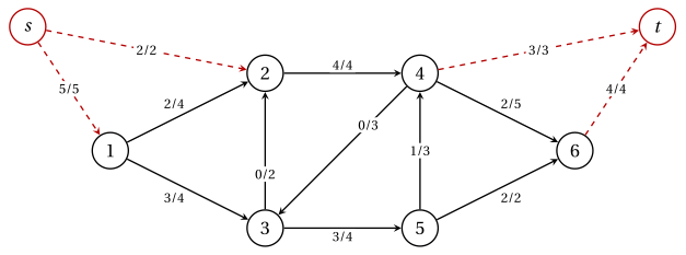
The restriction to \(A\) is \((2,3,4,0,3,0,2,1,2)\): on this instance it is the optimal flow \(\tilde{\vet{x}}\) of Chapter 4. This is a coincidence, since the search never looks at the costs.
A super source feeding the supply nodes and a super sink fed by the demand nodes turn feasibility into a maximum flow problem: the network has a feasible flow if and only if the maximum flow saturates all the new arcs.