6.7 The successive shortest path algorithm

Part 3 · Flows · Chapter 6 · Chapter 6: Minimum cost flow · Lecture notes, volume 3 (PDF) · Exercises: Minimum cost flow

Definition 6.15: pseudoflow and imbalances

A pseudoflow is a vector \(\vet{x}\) with \(\vet{l} \le \vet{x} \le \vet{u}\), which may violate flow conservation. The imbalance of node \(i\) is

\[ e_i=b_i-\Big(\sum_{(i,j) \in \delta^+(i)} x_{ij}-\sum_{(j,i) \in \delta^-(i)} x_{ji}\Big): \]

the supply that \(i\) has still to send if \(e_i>0\) (an excess node), the demand that it has still to receive if \(e_i<0\) (a deficit node).

• A pseudoflow is a feasible flow exactly when \(\vet{e}=\vet{0}\). The imbalances add up to zero, since the balances do and every arc adds \(x_{ij}\) to its tail and subtracts it from its head.

• The residual network \(G(\vet{x})\) of a pseudoflow is defined as in Definition 6.1. Augmenting \(\vet{x}\) along a path \(P\) of \(G(\vet{x})\) from \(s\) to \(t\) by \(\delta \le r(P)=\min_{(i,j) \in P}r_{ij}\) is defined as for cycles: the bounds still hold, \(e_s\) decreases by \(\delta\), \(e_t\) increases by \(\delta\), and the cost grows by \(\delta\, c(P)\), where \(c(P)=\sum_{(i,j) \in P} c^x_{ij}\).

• The idea is to keep potentials with non-negative reduced costs on \(G(\vet{x})\), the condition of Theorem 6.9, while the imbalances go to zero. With \(\vet{x}=\vet{0}\), \(\vet{\pi}= \vet{0}\) and costs \(c_{ij} \ge 0\) the condition holds at the start.

Lemma 6.16: shortest paths keep the reduced costs non-negative

Let \(\vet{x}\) be a pseudoflow and \(\vet{\pi}\) potentials with \(\bar{c}^{\pi}_{ij}=c^x_{ij}-\pi_i+\pi_j \ge 0\) on every arc of \(G(\vet{x})\). Let \(d(i)\) be the distances from a node \(s\) in \(G(\vet{x})\) with the lengths \(\bar{c}^{\pi}\) (\(d(i)=+\infty\) if \(i\) is not reachable), \(t\) a node with \(d(t)<+\infty\), \(P\) a shortest path from \(s\) to \(t\), and

\[ \pi'_i=\pi_i-\min\{d(i),d(t)\}, \qquad \forall i \in N . \]

• (a) \(c^x_{ij}-\pi'_i+\pi'_j \ge 0\) on every arc of \(G(\vet{x})\).

• (b) \(c^x_{ij}-\pi'_i+\pi'_j=0\) on every arc of \(P\).

• (c) If \(\vet{x}'\) is \(\vet{x}\) augmented along \(P\) by \(\delta \le r(P)\), then \(c^{x'}_{ij}-\pi'_i+\pi'_j \ge 0\) on every arc of \(G(\vet{x}')\).

Proof

Let \(\hat{d}(i)=\min\{d(i),d(t)\}\). The reduced cost of \((i,j)\) with \(\vet{\pi}'\) is \(\bar{c}^{\pi}_{ij}+\hat{d}(i)- \hat{d}(j)\).

• (a) Let \((i,j)\) be an arc of \(G(\vet{x})\). If \(d(i)<+\infty\), a shortest path to \(i\) followed by \((i,j)\) gives \(d(j) \le d(i)+\bar{c}^{\pi}_{ij}\), so \(\hat{d}(j) \le \min\{d(i)+\bar{c}^{\pi}_{ij},\,d(t)\} \le \hat{d}(i)+ \bar{c}^{\pi}_{ij}\), since \(\bar{c}^{\pi}_{ij} \ge 0\). If \(d(i)=+\infty\), then \(\hat{d}(i)=d(t) \ge \hat{d}(j)\). In both cases the new reduced cost is non-negative.

• (b) Subpaths of \(P\) are shortest (Lemma «optimality of subpaths» of Chapter 3), so \(d(j)=d(i)+ \bar{c}^{\pi}_{ij}\) on every arc of \(P\), and \(d(i) \le d(t)\) along \(P\) since the lengths are non-negative. Hence \(\hat{d}=d\) on \(P\), and the new reduced cost is \(0\).

• (c) Augmenting along \(P\) changes \(G(\vet{x})\) only on the arcs of \(P\): an arc \((i,j)\) of \(P\) may disappear, and the reverse arc \((j,i)\) may appear. The reverse of a residual arc has the opposite cost, hence by (b) reduced cost \(0\); the other arcs keep their reduced costs, non-negative by (a).

□

• For every path \(P\) from \(s\) to \(t\) the potentials telescope: \(\sum_{(i,j) \in P}\bar{c}^{\pi}_{ij}=c(P)-\pi_s+ \pi_t\). A shortest path for the reduced costs is a minimum cost path of \(G(\vet{x})\): the flow travels along cheapest paths, hence the name of the algorithm.

Algorithm: Successive shortest path algorithm

Input: a balanced network with \(\vet{l}=\vet{0}\), integer \(b_i\) and \(u_{ij}\), costs \(c_{ij} \ge 0\)

Output: an optimal flow \(\vet{x}\) with its certificate \(\vet{\pi}\), or «infeasible»

1Step 0 (initialization). Set \(\vet{x}:=\vet{0}\), \(\vet{\pi}:=\vet{0}\) and \(\vet{e}:=\vet{b}\).

2Step 1 (selection). If \(\vet{e}=\vet{0}\), STOP: \(\vet{x}\) is optimal, with \(\vet{\pi}\).

3 Otherwise let \(s\) be the node of smallest index with \(e_s>0\).

4Step 2 (shortest paths). Run Dijkstra from \(s\) on \(G(\vet{x})\), lengths \(c^x_{ij}-\pi_i+\pi_j\).

5 If no node with \(e_t<0\) is reachable, STOP: infeasible.

6 Otherwise \(t\) is the reachable node with \(e_t<0\) and smallest \(d(t)\), and \(P\) its path.

7Step 3 (augmentation). Set \(\pi_i:=\pi_i-\min\{d(i),d(t)\}\) for every \(i \in N\).

8 Augment \(\vet{x}\) along \(P\) by \(\delta:=\min\{e_s,-e_t,r(P)\}\), and update \(e_s\), \(e_t\).

9 Go to Step 1.

• Rules of this chapter. Dijkstra's algorithm breaks ties by the smallest index, as in Chapter 3; among the deficit nodes at the same distance, \(t\) is the one of smallest index.

Theorem 6.17: correctness of the successive shortest path algorithm

With the input of the algorithm, at the beginning of every iteration \(\vet{x}\) is an integer pseudoflow and \(c^x_{ij}-\pi_i+\pi_j \ge 0\) on every arc of \(G(\vet{x})\). The algorithm stops after at most \(D=\sum_{i: b_i>0}b_i\) iterations. If it stops in Step 1, \(\vet{x}\) is an optimal flow; if it stops in Step 2, the network has no feasible flow.

Proof

We prove the invariant, then the bound and the two stops.

1. Invariant. At the start \(G(\vet{0})\) has the forward arcs only, with costs \(c_{ij} \ge 0\), and \(\vet{\pi}=\vet{0}\). Dijkstra's algorithm applies, the lengths being non-negative, and Lemma 6.16(c) keeps the reduced costs non-negative. The amount \(\delta\) is a positive integer, since \(e_s\), \(-e_t\) and the residual capacities are positive integers (or \(+\infty\)), so \(\vet{x}\) stays integer.

2. Bound. If \(e_s>0\), some node has \(e_t<0\), since the imbalances add up to zero. Every iteration lowers \(\sum_{i: e_i>0}e_i\) by \(\delta \ge 1\), and no imbalance changes sign, since \(\delta \le e_s\) and \(\delta \le -e_t\). The sum starts at \(D\).

3. Stop in Step 1. \(\vet{e}=\vet{0}\), so \(\vet{x}\) is a feasible flow, optimal by the invariant and Theorem 6.9.

4. Stop in Step 2. Let \(S\) be the set of the nodes reachable from \(s\). No arc of \(G(\vet{x})\) leaves \(S\), so \(x_{ij}=u_{ij}\) on \(\delta^+(S)\) and \(x_{ij}=0\) on \(\delta^-(S)\). The pseudoflow satisfies conservation with the balances \(b_i-e_i\), so by Lemma «flow across a cut» of Chapter 4

   \[ \sum_{i \in S} b_i=x(\delta^+(S))-x(\delta^-(S))+\sum_{i \in S} e_i=u(\delta^+(S))+\sum_{i \in S}e_i>u(\delta^+(S)), \]

   because \(e_s>0\) and no node of \(S\) has \(e_i<0\). The cut condition of Chapter 4 fails for \(S\): there is no feasible flow.

□

• Running time. Each iteration runs Dijkstra's algorithm in \(O(n^2)\) time: \(O(D\,n^2)\) in total, a pseudo-polynomial bound.

• Negative costs. If some arcs with finite capacity have \(c_{ij}<0\), start from \(x_{ij}=u_{ij}\) on them and \(x_{ij}=0\) elsewhere, with \(\vet{e}=\vet{b}-\mat{B}\vet{x}\): such an arc gives only its backward arc, of cost \(-c_{ij}>0\), and \(\vet{\pi}=\vet{0}\) works again.

6.7.1 Successive shortest paths on the reference network

Example 6.7: successive shortest paths

We start from \(\vet{x}=\vet{0}\), \(\vet{\pi}=\vet{0}\) and \(\vet{e}=\vet{b}=(5,2,0,-3,0,-4)\). In the first table each row is an iteration, with the node \(s\), the distances of Dijkstra's algorithm and the node \(t\); the second table gives the path \(P\), its reduced cost \(d(t)\) and its cost \(c(P)\), the amount \(\delta\) and the cost of the new flow.

it.	\(s\)	\(d(1)\)	\(d(2)\)	\(d(3)\)	\(d(4)\)	\(d(5)\)	\(d(6)\)	\(t\)
\(1\)	\(1\)	\(0\)	\(2\)	\(2\)	\(7\)	\(5\)	\(8\)	\(4\)
\(2\)	\(1\)	\(0\)	\(0\)	\(0\)	\(0\)	\(0\)	\(1\)	\(6\)
\(3\)	\(2\)	\(0\)	\(0\)	\(0\)	\(0\)	\(0\)	\(4\)	\(6\)
\(4\)	\(2\)	\(0\)	\(0\)	\(0\)	\(3\)	\(0\)	\(3\)	\(6\)

it.	\(P\)	\(d(t)\)	\(c(P)\)	\(\delta\)	cost
\(1\)	\(1,2,4\)	\(7\)	\(7\)	\(3\)	\(21\)
\(2\)	\(1,3,5,6\)	\(1\)	\(8\)	\(2\)	\(37\)
\(3\)	\(2,4,6\)	\(4\)	\(10\)	\(1\)	\(47\)
\(4\)	\(2,1,3,5,4,6\)	\(3\)	\(13\)	\(1\)	\(60\)

The third table gives, after each iteration, the potentials, the imbalances and the flow.

it.	\(\vet{\pi}\)	\(\vet{e}\)	\(\vet{x}\)
\(0\)	\((0,0,0,0,0,0)\)	\((5,2,0,-3,0,-4)\)	\((0,0,0,0,0,0,0,0,0)\)
\(1\)	\((0,-2,-2,-7,-5,-7)\)	\((2,2,0,0,0,-4)\)	\((3,0,3,0,0,0,0,0,0)\)
\(2\)	\((0,-2,-2,-7,-5,-8)\)	\((0,2,0,0,0,-2)\)	\((3,2,3,0,2,0,0,0,2)\)
\(3\)	\((0,-2,-2,-7,-5,-12)\)	\((0,1,0,0,0,-1)\)	\((3,2,4,0,2,0,1,0,2)\)
\(4\)	\((0,-2,-2,-10,-5,-15)\)	\((0,0,0,0,0,0)\)	\((2,3,4,0,3,0,2,1,2)\)

The reduced costs \(\bar{c}_{ij}=c_{ij}-\pi_i+\pi_j\) of the arcs of \(A\), before each iteration, are (the forward arc has \(\bar{c}_{ij}\) if \(x_{ij}<u_{ij}\), the backward arc \(-\bar{c}_{ij}\) if \(x_{ij}>0\)):

it.	\((1,2)\)	\((1,3)\)	\((2,4)\)	\((3,2)\)	\((3,5)\)	\((4,3)\)	\((4,6)\)	\((5,4)\)	\((5,6)\)
\(1\)	\(2\)	\(2\)	\(5\)	\(2\)	\(3\)	\(3\)	\(5\)	\(5\)	\(3\)
\(2\)	\(0\)	\(0\)	\(0\)	\(2\)	\(0\)	\(8\)	\(5\)	\(3\)	\(1\)
\(3\)	\(0\)	\(0\)	\(0\)	\(2\)	\(0\)	\(8\)	\(4\)	\(3\)	\(0\)
\(4\)	\(0\)	\(0\)	\(0\)	\(2\)	\(0\)	\(8\)	\(0\)	\(3\)	\(-4\)

• Iteration \(1\). The reduced costs are the costs. The deficit nodes \(4\) and \(6\) are at distance \(7\) and \(8\): \(t=4\), and \(\delta=\min\{5,3,4,4\}=3\). Node \(6\) is farther than \(t\) and its potential decreases by \(7\), not \(8\).

• Iteration \(2\). The arcs \((1,2)\), \((2,4)\) of the first path now have reduced cost \(0\), and so do their backward arcs. The path \(1,3,5,6\) has reduced cost \(1\) and cost \(8\); \(\delta=\min\{2,4,4,4,2\}=2\) is set by \(e_1\) and by \(u_{56}\).

• Iteration \(3\). \(s=2\), and \(d(1)=0\) through the backward arc \((2,1)\). The path \(2,4,6\) uses the last unit of \((2,4)\).

• Iteration \(4\). The path \(2,1,3,5,4,6\) uses the backward arc \((2,1)\): one unit that went from \(1\) to \(2\) is rerouted from \(1\) through \(3\), \(5\) and \(4\). The figure shows \(G(\vet{x})\) with \(r_{ij}\) and the reduced cost on each arc, and the path in blue.

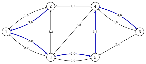
After iteration \(4\) the imbalances are zero and \(\vet{x}=\tilde{\vet{x}}\), of cost \(60\). Shifted by \(15\), the potentials become \((15,13,13,5,10,0)\): the potentials of Chapter 4.

• Here the costs \(7,8,10,13\) of the paths grow from one iteration to the next: later units travel along more expensive paths, and the total cost is \(3 \cdot 7+2 \cdot 8+10+13=60\).

• Four iterations are enough here, while the bound of Theorem 6.17 is \(D=7\).

Dijkstra needs the reduced costs

In iteration \(4\) the arcs \((2,1)\), \((3,1)\), \((4,2)\), \((5,3)\), \((6,4)\), \((6,5)\) of \(G(\vet{x})\) are backward arcs with negative costs \(c^x_{ij}\), and Dijkstra's algorithm with negative lengths can fail (Chapter 3). The potentials make all the lengths non-negative without changing the shortest paths.

The successive shortest path algorithm sends flow from an excess node to a deficit node along a shortest path of \(G(\vet{x})\), found by Dijkstra's algorithm on the reduced costs. The update \(\pi_i:=\pi_i-\min\{d(i),d(t)\}\) keeps the reduced costs non-negative, so the final flow is optimal and the potentials certify it.

6.8 Typical mistakes

Warning

• Giving the backward arc the cost \(+c_{ij}\). A backward arc decreases \(x_{ij}\), so it saves \(c_{ij}\) per unit: its cost is \(-c_{ij}\), and its residual capacity is \(x_{ij}-l_{ij}\).

• Augmenting by more than \(r(W)\). Some arc of the cycle would leave its bounds; \(\theta=r(W)\) is the largest step.

• Running Bellman–Ford from a single node. A negative cycle that is not reachable from that node is missed; the labels start at \(0\) on every node.

• Taking the walk for the cycle. The walk with \(n\) arcs read from the table contains a negative cycle, but it is not a cycle itself: the cycle is the piece between two occurrences of the same node.

• Running Dijkstra's algorithm on the costs \(c^x_{ij}\). Backward arcs can have negative costs; the lengths are the reduced costs \(c^x_{ij}-\pi_i+\pi_j\).

• Updating the potentials with the wrong sign. With \(\bar{c}_{ij}=c_{ij}-\pi_i+\pi_j\) the update is \(\pi_i:=\pi_i-\min\{d(i),d(t)\}\); the nodes farther than \(t\) decrease by \(d(t)\) only.

• Taking the maximum flow of Step 0 as optimal. The auxiliary network has no costs: its maximum flow is feasible, and optimal only by chance.

6.9 In summary

In summary

• The residual network \(G(\vet{x})\) has a forward arc \((i,j)\) with \(r_{ij}=u_{ij}-x_{ij}\) and cost \(c_{ij}\), and a backward arc \((j,i)\) with \(r_{ji}=x_{ij}-l_{ij}\) and cost \(-c_{ij}\); augmenting along a cycle \(W\) changes the cost by \(\theta\,c(W)\).

• A circulation decomposes into cycles; the difference of two feasible flows is a circulation on \(G(\vet{x})\).

• A feasible flow is optimal if and only if \(G(\vet{x})\) has no negative cycle, if and only if some potentials give non-negative reduced costs on \(G(\vet{x})\); on the arcs of \(A\): \(\bar{c}_{ij}>0 \Rightarrow x_{ij}=l_{ij}\), \(\bar{c}_{ij}<0 \Rightarrow x_{ij}=u_{ij}\).

• A maximum flow from a super source to a super sink finds a feasible flow or proves that there is none.

• Cycle canceling: Bellman–Ford from labels \(0\) finds a negative cycle, augmenting by \(r(W)\) cancels it; at most \(\vet{c}'\vet{x}^0-z(\mathrm{MCF})\) iterations with integer data.

• Successive shortest paths: Dijkstra on the reduced costs from an excess node to the nearest deficit node, \(\pi_i:=\pi_i-\min\{d(i),d(t)\}\); at most \(D\) iterations.

The reference network at a glance.

most expensive flow	\(\vet{x}^0=(1,4,4,1,4,1,3,3,1)\), cost \(80\)
cycle canceling from \(\vet{x}^0\)	cycles \(4,5,3,4\); \(6,4,5,6\); \(3,1,2,3\): costs \(80,69,62,60\)
successive shortest paths	paths \(1,2,4\); \(1,3,5,6\); \(2,4,6\); \(2,1,3,5,4,6\): costs \(21,37,47,60\)
first feasible flow	maximum flow of value \(7\); on \(A\) it is \(\tilde{\vet{x}}\)
optimal flow	\(\tilde{\vet{x}}=(2,3,4,0,3,0,2,1,2)\), \(z(\mathrm{MCF})=60\)
potentials (\(\pi_6=0\))	\(\vet{\pi}=(15,13,13,5,10,0)\)

---

Exercises on this chapter: Minimum cost flow