7.3 Initial basic feasible solutions

Part 3 · Flows · Chapter 7 · Chapter 7: Transportation and assignment · Lecture notes, volume 3 (PDF) · Exercises: Transportation and assignment

• A basic feasible solution is built by filling the tableau one cell at a time. A row or a column is active until it is crossed out; the residual supply \(\bar{a}_i\) and the residual demand \(\bar{d}_j\) are what is left to ship and to receive.

• The two rules below differ only in the choice of the next cell.

Algorithm: Initial basic feasible solution

Input: a balanced instance with supplies \(a_i\), demands \(d_j\) and costs \(c_{ij}\)

Output: a basis \(T\) and its basic feasible solution \(\bar{\vet{x}}\)

1Step 0 (initialization). All rows and columns are active; \(\bar{a}_i:=a_i\), \(\bar{d}_j:=d_j\), \(T:=\emptyset\).

2Step 1 (choice of the cell). Choose a cell \((i,j)\) with active row and column:

3 north-west corner rule: the cell with the smallest \(i\) and the smallest \(j\);

4 minimum cost rule: the cell with the smallest \(c_{ij}\) (the smallest \(i\), then \(j\), on ties).

5Step 2 (amount). Set \(\bar{x}_{ij}:=\min\{\bar{a}_i,\bar{d}_j\}\), add \((i,j)\) to \(T\), and subtract \(\bar{x}_{ij}\) from \(\bar{a}_i\) and from \(\bar{d}_j\).

6Step 3 (crossing out). If \(\bar{a}_i=0\) and another row is active, cross out row \(i\); otherwise cross out column \(j\).

7 If no column is active, STOP; otherwise go to Step 1.

• When \(\bar{a}_i=\bar{d}_j=0\) at the same time, only the row is crossed out: the column stays active with residual demand \(0\), and a later cell of that column gets the amount \(0\). This basic cell with value \(0\) keeps \(T\) a spanning tree, and the solution is degenerate.

Theorem 7.8: the initial solution is basic

With either rule, the algorithm «Initial basic feasible solution» stops after \(m+n-1\) steps, and \(T\) is a basis with basic feasible solution \(\bar{\vet{x}}\).

Proof

1. Invariant. The residual supplies of the active rows and the residual demands of the active columns have equal sums: true at the start, and Step 2 subtracts the same amount from both sides.

2. A crossed line has residual \(0\). A crossed row has \(\bar{a}_i=0\). A column is crossed when \(\bar{a}_i>0\), and then \(\bar{x}_{ij}=\bar{d}_j\) and \(\bar{d}_j=0\), or when row \(i\) is the only active row with \(\bar{a}_i=0\), and then every active column has residual \(0\) by the invariant.

3. Counting. A row is crossed out only if another row is active, so one row \(r\) is never crossed out, and the algorithm stops when the \(n\) columns are crossed out. At the stop the active rows have residual \(0\) by the invariant, and a row that reaches \(0\) without being crossed out is the only active row. Hence the steps are \((m-1)+n=m+n-1\), one cell each, all different, since a cell is chosen in two active lines and one of them is then crossed out.

4. Feasibility. At the stop every row and every column has residual \(0\), so \(\bar{\vet{x}} \ge \vet{0}\) satisfies all the constraints.

5. Tree. Let \(L_t\) be the line crossed at step \(t\): no later cell lies in \(L_t\). Backwards from the last step, the cells of steps \(t,t+1,\dots\) form a tree: the cell of step \(t\) joins the new node \(L_t\) to its other line, which is still active, hence a node of the later cells or the row \(r\). At \(t=1\) the tree spans all the \(m+n\) nodes. □

7.3.1 The north-west corner rule

Example 7.5: the north-west corner rule

On Example 7.1 the north-west corner rule starts at the cell \((1,4)\) and moves right or down. Its steps are:

step	cell	amount	crossed out
\(1\)	\((1,4)\)	\(10\)	column \(4\)
\(2\)	\((1,5)\)	\(20\)	row \(1\)
\(3\)	\((2,5)\)	\(5\)	column \(5\)
\(4\)	\((2,6)\)	\(15\)	column \(6\)
\(5\)	\((2,7)\)	\(10\)	row \(2\)
\(6\)	\((3,7)\)	\(30\)	row \(3\), column \(7\)

The basic feasible solution, with the basic cells in blue, is

\(\bar{x}_{ij}\)	\(4\)	\(5\)	\(6\)	\(7\)	\(a_i\)
\(1\)	\(10\)	\(20\)			\(30\)
\(2\)		\(5\)	\(15\)	\(10\)	\(30\)
\(3\)				\(30\)	\(30\)
\(d_j\)	\(10\)	\(25\)	\(15\)	\(40\)

Its cost is

\[ 1 \cdot 10+9 \cdot 20+4 \cdot 5+2 \cdot 15+2 \cdot 10+6 \cdot 30=440 . \]

The six basic cells form the spanning tree below, with the amounts on the arcs.

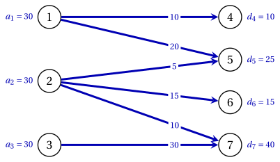
• The north-west corner rule ignores the costs: on this instance it ships \(20\) units on the cell \((1,5)\), of cost \(9\), and \(30\) units on \((3,7)\), of cost \(6\).

7.3.2 The minimum cost rule

Example 7.6: the minimum cost rule

On Example 7.1 the minimum cost rule chooses, at every step, the cheapest cell of the active rows and columns:

step	cell	amount	crossed out
\(1\)	\((1,4)\)	\(10\)	column \(4\)
\(2\)	\((3,5)\)	\(25\)	column \(5\)
\(3\)	\((1,6)\)	\(15\)	column \(6\)
\(4\)	\((2,7)\)	\(30\)	row \(2\)
\(5\)	\((1,7)\)	\(5\)	row \(1\)
\(6\)	\((3,7)\)	\(5\)	row \(3\), column \(7\)

• At step \(1\) the cells \((1,4)\) and \((3,5)\) both cost \(1\), and \((1,4)\) goes first, since its row is smaller. At step \(3\) the cells \((1,6)\), \((2,6)\), \((2,7)\) cost \(2\), and \((1,6)\) goes first.

• At step \(4\) only column \(7\) is active: it takes the whole supply of row \(2\), then \(5\) units from row \(1\) and \(5\) from row \(3\).

The basic feasible solution is

\(\bar{x}_{ij}\)	\(4\)	\(5\)	\(6\)	\(7\)	\(a_i\)
\(1\)	\(10\)		\(15\)	\(5\)	\(30\)
\(2\)				\(30\)	\(30\)
\(3\)		\(25\)		\(5\)	\(30\)
\(d_j\)	\(10\)	\(25\)	\(15\)	\(40\)

with cost

\[ 1 \cdot 10+2 \cdot 15+3 \cdot 5+2 \cdot 30+1 \cdot 25+6 \cdot 5=170 . \]

Filling one cell per step and crossing out one line per step gives a basic feasible solution with \(m+n-1\) basic cells. The north-west corner rule ignores the costs; the minimum cost rule usually starts much closer to the optimum (\(170\) instead of \(440\) on the example).

---

Next: 7.4 The potential method