7.1 The transportation problem

Part 3 · Flows · Chapter 7 · Chapter 7: Transportation and assignment · Lecture notes, volume 3 (PDF) · Exercises: Transportation and assignment

Definition 7.1: transportation problem

There are \(m\) origins and \(n\) destinations. We number the origins \(1,2,\dots,m\) and the destinations \(m+1,m+2,\dots,m+n\), and we write

\[ P=\{1,2,\dots,m\}, \qquad D=\{m+1,m+2,\dots,m+n\}. \]

• Every origin \(i \in P\) has a supply \(a_i>0\), every destination \(j \in D\) has a demand \(d_j>0\), and \(c_{ij} \in \R\) is the cost of shipping one unit from \(i\) to \(j\).

• The instance is balanced if \(\sum_{i \in P} a_i=\sum_{j \in D} d_j\).

The transportation problem asks for the amounts \(x_{ij} \ge 0\) to ship from every origin \(i\) to every destination \(j\), so that every origin ships its whole supply and every destination receives its demand, at minimum total cost.

• In this chapter \(m\) and \(n\) are the numbers of origins and destinations. The underlying network has \(m+n\) nodes and one arc \((i,j)\) for every \(i \in P\) and \(j \in D\), that is \(m\,n\) arcs: it is the complete bipartite network of \(P\) and \(D\), since every arc goes from \(P\) to \(D\).

• Numbering the destinations after the origins gives every node its own number, and later its own potential.

• We use one continuous variable \(x_{ij}\) for every pair \(i \in P\), \(j \in D\): the amount shipped from \(i\) to \(j\).

Using these variables, an LP model for the transportation problem reads as follows:

\[\begin{align*} && \min \;\;{\sum_{i \in P} \sum_{j \in D} c_{ij} \, x_{ij}} \label{ta:obj} \tag{7.1a}\\[1ex] && \text{subject to} \quad \sum_{j \in D} x_{ij} &= a_i, & \forall i \in P, \label{ta:supply} \tag{7.1b}\\[1ex] && \sum_{i \in P} x_{ij} &= d_j, & \forall j \in D, \label{ta:demand} \tag{7.1c}\\[1ex] && x_{ij} &\ge 0, & \forall i \in P,~\forall j \in D. \label{ta:dom} \tag{7.1d} \end{align*}\]

This LP model is referred to as the \(\mathrm{TP}\) model.

• Description of the objective function and constraints of the \(\mathrm{TP}\) model:

  • the objective function \(\eqref{ta:obj}\) minimizes the total shipping cost;

  • constraints \(\eqref{ta:supply}\), one for every origin, ship the whole supply of the origin;

  • constraints \(\eqref{ta:demand}\), one for every destination, deliver the whole demand of the destination;

  • finally, constraints \(\eqref{ta:dom}\) define the variables of the LP model.

• Multiplying the constraints \(\eqref{ta:demand}\) by \(-1\) gives the flow conservation constraints of the complete bipartite network, with balances \(b_i=a_i\) for \(i \in P\), \(b_j=-d_j\) for \(j \in D\), and no capacities. The \(\mathrm{TP}\) model is the \(\mathrm{MCF}\) model of the row «Transportation» of the table «Special cases» of Chapter 4 «Network flow models».

Proposition 7.2: feasibility and integrality

An instance of the transportation problem has a feasible solution if and only if it is balanced. A balanced instance has an optimal solution, and if the supplies \(a_i\) and the demands \(d_j\) are integer, it has an integer optimal solution.

Proof

Let \(S=\sum_{i \in P} a_i\).

1. Balance is necessary. If \(\vet{x}\) is feasible, adding up the constraints \(\eqref{ta:supply}\) and the constraints \(\eqref{ta:demand}\) gives the same sum of all the variables: \(\sum_{i \in P} a_i=\sum_{i \in P}\sum_{j \in D} x_{ij}=\sum_{j \in D} d_j\).

2. Balance is sufficient. If \(S=\sum_{j \in D} d_j\), the amounts \(x_{ij}=a_i\,d_j/S \ge 0\) are feasible: row \(i\) adds up to \(a_i\sum_{j \in D} d_j/S=a_i\), and column \(j\) to \(d_j\sum_{i \in P} a_i/S=d_j\).

3. Optimal solution. Every feasible solution has \(0 \le x_{ij} \le a_i\), so the feasible region is a nonempty bounded polyhedron, and a linear function attains its minimum over it at a vertex (Chapter 15 «The geometry of Linear Programming» of the module Linear Programming).

4. Integrality. With integer balances and no capacities, every vertex is integer by the Theorem «integer vertices» of Chapter 4. □

7.1.1 The transportation tableau

• The transportation tableau is an \(m \times n\) table with one row for every origin and one column for every destination. The cell \((i,j)\) holds the cost \(c_{ij}\), or later the amount \(x_{ij}\); the last column holds the supplies \(a_i\) and the last row the demands \(d_j\).

• A vector \(\vet{x} \ge \vet{0}\) written in the tableau is feasible if and only if every row adds up to its supply and every column to its demand.

Example 7.1: three warehouses and four stores

A company has three warehouses, the origins \(1,2,3\), with \(30\) units each, and four stores, the destinations \(4,5,6,7\), with demands \(10\), \(25\), \(15\) and \(40\). The unit costs are in the tableau:

\[ \begin{array}{c|cccc|c} \hline {c_{ij}} & {4} & {5} & {6} & {7} & {a_i} \\ \hline {1} & {1} & {9} & {2} & {3} & {30} \\ {2} & {3} & {4} & {2} & {2} & {30} \\ {3} & {9} & {1} & {4} & {6} & {30} \\ \hline {d_j} & {10} & {25} & {15} & {40} & {90} \\ \hline \end{array} \]

The instance is balanced: the total supply and the total demand are both \(90\). In the complete bipartite network every origin is joined to every destination, with \(3 \cdot 4=12\) arcs; next to each node, its supply or its demand.

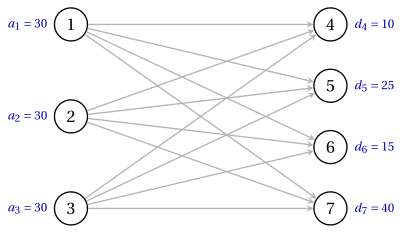
The proportional amounts \(x_{ij}=a_i\,d_j/90\) of Proposition 7.2 are feasible, for example \(x_{14}=30 \cdot 10/90=\frac{10}{3}\), but fractional; the vertices of the feasible region are integer.

7.1.2 Unbalanced instances

• If the total supply exceeds the total demand and every origin ships at most its supply, we add a dummy destination with demand \(\sum_{i \in P} a_i-\sum_{j \in D} d_j\) and cost \(0\) from every origin. The amount shipped to it is the unused supply of the origin: this is the dummy node of Chapter 4, as a column of the tableau.

• If the total demand exceeds the total supply and a destination may receive less than its demand, we add a dummy origin with supply \(\sum_{j \in D} d_j-\sum_{i \in P} a_i\). The cost of its cell \((\cdot,j)\) is the penalty for each unit of unmet demand of \(j\), or \(0\) if there is none.

Example 7.2: a dummy destination

In Example 7.1 the supply of warehouse \(1\) grows to \(a_1=40\): the total supply is \(100\) and the total demand \(90\).

• We add the dummy destination \(8\) with demand \(d_8=100-90=10\), and the cells \((1,8)\), \((2,8)\), \((3,8)\) with cost \(0\): the tableau has a fifth column.

• The optimal solution, computed with Gurobi, is unique:

  \[ \tilde{x}_{14}=10,~ \tilde{x}_{16}=15,~ \tilde{x}_{17}=10,~ \tilde{x}_{18}=5,~ \tilde{x}_{27}=30,~ \tilde{x}_{35}=25,~ \tilde{x}_{38}=5, \]

  with cost \(155\). Warehouses \(1\) and \(3\) keep \(5\) units each, and warehouse \(2\) ships all its supply.

7.1.3 Transshipment as transportation

• In a transshipment instance the units may pass through intermediate nodes. When the arcs have no capacities, every unit can travel along a shortest path, and only the distances between supply and demand nodes matter.

Proposition 7.3: transshipment as transportation

Let \(G=(N,A)\) be a network with balances \(b_i\), zero lower bounds, no capacities and costs \(c_{ij} \ge 0\). Let \(P=\{i \in N : b_i>0\}\) and \(D=\{j \in N : b_j<0\}\), and assume that every \(j \in D\) is reachable from every \(i \in P\), with distance \(\tilde{d}(i,j)\) for the lengths \(c_{ij}\). Then the minimum cost of a feasible flow equals the optimal value of the transportation instance with origins \(P\), supplies \(a_i=b_i\), destinations \(D\), demands \(d_j=-b_j\) and costs \(\tilde{d}(i,j)\).

Proof

We compare the two optimal values.

1. From shipments to flows. Let \(\vet{y}\) be feasible for the transportation instance. Sending \(y_{ij}\) units along a shortest path from \(i\) to \(j\), for every pair, gives a flow \(\vet{x} \ge \vet{0}\): node \(i \in P\) sends \(\sum_{j \in D} y_{ij}=b_i\) units, node \(j \in D\) receives \(-b_j\), the other nodes pass on what they receive. Its cost is \(\sum_{i,j} \tilde{d}(i,j)\,y_{ij}\), so the minimum flow cost is at most the transportation optimum.

2. From flows to shipments. We show by induction on the number of arcs with \(x_{ij}>0\) plus the number of nodes with \(b_i \neq 0\) that every feasible flow \(\vet{x}\) costs at least \(\sum_{i,j} \tilde{d}(i,j)\,y_{ij}\) for some feasible \(\vet{y}\). If \(\vet{b}=\vet{0}\), take \(\vet{y}=\vet{0}\).

3. Otherwise start at a node \(i_0\) with \(b_{i_0}>0\): its outflow is positive, so it has a leaving arc with positive flow. A node \(v\) with \(b_v \ge 0\) reached along such an arc has a positive inflow, hence a positive outflow. Follow these arcs until a node repeats or a node \(j_0\) with \(b_{j_0}<0\) is reached.

4. If a node repeats, the arcs form a directed cycle \(C\) with positive flows. Subtracting their minimum \(\varepsilon\) along \(C\) keeps the flow feasible, does not increase the cost, since \(c \ge 0\), and empties an arc: the induction applies.

5. Otherwise we have a path \(Q\) from \(i_0\) to \(j_0\). Let \(\varepsilon>0\) be the minimum of \(b_{i_0}\), \(-b_{j_0}\) and the flows on \(Q\). Subtracting \(\varepsilon\) along \(Q\), and from \(b_{i_0}\) and \(-b_{j_0}\), gives a feasible flow \(\vet{x}'\) for the new balances, with fewer positive arcs or nonzero balances, and

   \[ \vet{c}'\vet{x}=\vet{c}'\vet{x}'+\varepsilon\, c(Q) \ge \vet{c}'\vet{x}'+\varepsilon\,\tilde{d}(i_0,j_0). \]

   By induction \(\vet{c}'\vet{x}' \ge \sum \tilde{d}(i,j)\,y'_{ij}\); adding \(\varepsilon\) to \(y'_{i_0j_0}\) gives the required \(\vet{y}\).

□

Example 7.3: the transshipment instance of Chapter 4 without capacities

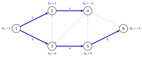
We take the reference network of Chapter 4, with the same balances \(\vet{b}=(5,2,0,-3,0,-4)\) and costs, and remove the capacities. The origins are the supply nodes \(1,2\) and the destinations the demand nodes \(4,6\); we keep the names of the network.

• The distances are \(\tilde{d}(1,4)=7\) along \(1,2,4\), \(\tilde{d}(1,6)=8\) along \(1,3,5,6\), \(\tilde{d}(2,4)=5\) along \(2,4\), and \(\tilde{d}(2,6)=10\) along \(2,4,6\).

• The \(2 \times 2\) transportation instance has \(a_1=5\), \(a_2=2\), \(d_4=3\), \(d_6=4\). With \(y_{24}=t \in [0,2]\) the other amounts are \(y_{14}=3-t\), \(y_{16}=2+t\), \(y_{26}=2-t\), and the cost is

  \[ 7(3-t)+8(2+t)+5t+10(2-t)=57-4t, \]

  minimum for \(t=2\): \(y_{14}=1\), \(y_{16}=4\), \(y_{24}=2\), \(y_{26}=0\), with cost \(49\).

• Along the shortest paths this gives the flow \(x_{12}=1\), \(x_{13}=4\), \(x_{24}=3\), \(x_{35}=4\), \(x_{56}=4\) (blue), of cost \(49\), the optimum computed by Gurobi. With the capacities of Chapter 4 this flow is not feasible, since the arc \((5,6)\) has capacity \(2\), and the optimum is \(60\).

The transportation problem ships the supplies of \(m\) origins to the demands of \(n\) destinations at minimum cost. It is a minimum cost flow model on the complete bipartite network; it is feasible exactly when it is balanced, and a dummy origin or destination balances it.

---

Next: 7.2 Basic solutions