2.6 Prim's algorithm
Part 2 · Trees and paths · Chapter 2 · Chapter 2: Spanning trees · Lecture notes, volume 2 (PDF) · Exercises: Spanning trees · App: Minimum spanning trees: Kruskal and Prim
- Prim's algorithm grows a single tree from a start vertex \(s\): the set \(S\) of the vertices of the tree defines the cut \(\delta(S)\) of Step 2, and the lightest edge of the cut is found through a label \(d(v)\) for every vertex \(v \notin S\).
Algorithm: Prim's algorithm
STOP. Otherwise select \(v \notin S\) with minimum \(d(v)\), and set
\(S:=S \cup \{v\}\), \(F:=F \cup \{\{\mathit{pred}(v),v\}\}\).- In this module the start vertex is \(s=1\), and ties in Step 1 are broken by the smallest index.
Lemma 2.12: meaning of the labels
At every execution of Step 1 of Prim's algorithm, for every \(v \notin S\),
(\(+\infty\) if \(v\) has no neighbour in \(S\)), and when \(d(v)<+\infty\) the minimum is attained by \(u=\mathit{pred}(v)\).
Proof
By induction. At the first execution \(S=\{s\}\), and Step 0 sets exactly \(d(v)=w_{sv}\), or \(+\infty\). Assume the claim before the insertion of a vertex \(v\) into \(S\). For \(u \notin S \cup \{v\}\), the new set \(S \cup \{v\}\) adds the candidate \(w_{vu}\) when \(\{v,u\} \in E\), and Step 2 replaces \(d(u)\) and \(\mathit{pred}(u)\) exactly when this candidate is smaller. The other labels and predecessors are unchanged. □
Theorem 2.13: correctness of Prim's algorithm
Prim's algorithm stops with \(|F|=n-1\), and \(F\) is a minimum spanning tree.
Proof
All the edges of \(F\) have both endpoints in \(S\), so \(F \cap \delta(S)=\emptyset\).
-
By Lemma 2.12, \(\min_{v \notin S} d(v)\) is the minimum weight of an edge of \(\delta(S)\), attained by \(\{\mathit{pred}(v),v\}\) for the selected \(v\); it is finite because \(G\) is connected.
-
Hence every iteration is a choice of Step 2 of the generic greedy algorithm, with the cut \(\delta(S)\).
-
Each iteration adds one vertex to \(S\) and one edge to \(F\), so the algorithm stops after \(n-1\) iterations with \(|F|=n-1\); Theorem 2.9 concludes. □
Theorem 2.14: running time of Prim's algorithm
With the labels stored in an array, Prim's algorithm runs in \(O(n^2)\) time.
Proof
There are \(n-1\) selections, and each scans the labels of at most \(n\) vertices: \(O(n^2)\) in total. The update after the insertion of \(v\) scans the adjacency list of \(v\) in \(O(\deg(v))\) time, and \(\sum_{v \in V} \deg(v)=2m\). The total is \(O(n^2+m)=O(n^2)\), since \(m \le n^2\). □
-
On dense graphs, with \(m\) of the order of \(n^2\), the bound \(O(n^2)\) is linear in the size of the graph.
-
With the labels in a binary heap, each selection and each update take \(O(\log n)\) time, for \(O(m\log n)\) in total: better on sparse graphs.
2.6.1 Prim's algorithm on the reference graph
Example 2.8: Prim's algorithm from vertex \(1\)
We run Prim's algorithm on the weighted reference graph from \(s=1\). Each row shows the selected vertex, the edge added to \(F\) and the labels \(d(v)\) of the vertices outside \(S\) after the update, with \(\mathit{pred}(v)\) in brackets; a dash marks the vertices already in \(S\).
| iteration | selected | added edge | \(d(2)\) | \(d(3)\) | \(d(4)\) | \(d(5)\) | \(d(6)\) |
|---|---|---|---|---|---|---|---|
| \(0\) | \(1\) | – | \(4~(1)\) | \(1~(1)\) | \(\infty\) | \(\infty\) | \(\infty\) |
| \(1\) | \(3\) | \(\{1,3\}\) | \(3~(3)\) | – | \(5~(3)\) | \(8~(3)\) | \(\infty\) |
| \(2\) | \(2\) | \(\{2,3\}\) | – | – | \(5~(3)\) | \(8~(3)\) | \(\infty\) |
| \(3\) | \(4\) | \(\{3,4\}\) | – | – | – | \(2~(4)\) | \(9~(4)\) |
| \(4\) | \(5\) | \(\{4,5\}\) | – | – | – | – | \(7~(5)\) |
| \(5\) | \(6\) | \(\{5,6\}\) | – | – | – | – | – |
At iteration \(1\) the label of \(2\) drops from \(4\) to \(3\), because \(w_{32}=3<4\); at iteration \(3\) the label of \(5\) drops from \(8\) to \(2\). The figure shows the state after iteration \(2\): the cut \(\delta(\{1,2,3\})\) is crossed by \(\{2,4\}\), \(\{3,4\}\), \(\{3,5\}\), and the next edge is \(\{3,4\}\), with \(d(4)=5\).
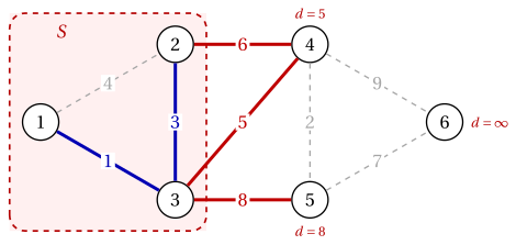
The final tree is \(\{1,3\},\{2,3\},\{3,4\},\{4,5\},\{5,6\}\), of weight \(18\): the same tree as Kruskal's algorithm, with the edges added in a different order.
- Kruskal's algorithm adds \(\{4,5\}\) second, while Prim's algorithm adds it fourth: Kruskal grows a forest, Prim a single tree containing \(s\).
Prim's algorithm grows one tree from \(s\) and adds the lightest edge leaving it; the labels \(d(v)\) give that edge in \(O(n)\) time, for \(O(n^2)\) in total.