5.1 The maximum flow problem

Part 3 · Flows · Chapter 5 · Chapter 5: Maximum flow · Lecture notes, volume 3 (PDF) · Exercises: Maximum flow · App: Maximum flow: Ford–Fulkerson and Edmonds–Karp

Definition 5.1: maximum flow problem

Let \(G=(N,A)\) be a directed graph with \(n=|N|\) nodes and \(m=|A|\) arcs, two distinct nodes \(s\), the source, and \(t\), the sink, and a capacity \(u_{ij} \ge 0\) for every arc \((i,j) \in A\).

• A feasible flow is a vector \(\vet{x} \in \R^m\) with \(0 \le x_{ij} \le u_{ij}\) for every arc \((i,j) \in A\) and flow conservation at every node other than \(s\) and \(t\):

  \[ \sum_{(i,j) \in \delta^+(i)} x_{ij} \;-\; \sum_{(j,i) \in \delta^-(i)} x_{ji}=0, \quad \forall i \in N \setminus \{s,t\}. \]

• The value of the flow is the net outflow of the source:

  \[ v=\sum_{(s,j) \in \delta^+(s)} x_{sj} \;-\; \sum_{(j,s) \in \delta^-(s)} x_{js} . \]

• The maximum flow problem asks for a feasible flow of maximum value, a maximum flow. Its value is denoted by \(\tilde{v}\).

• The capacities are finite, and the flow \(\vet{x}=\vet{0}\), of value \(0\), is always feasible.

• The nodes other than \(s\) and \(t\) pass on everything they receive: the flow leaves \(s\) and travels through the network towards \(t\).

• As in Chapter 4 «Network flow models», \(\delta^+(i)\) and \(\delta^-(i)\) are the arcs leaving and entering node \(i\), and the arcs are numbered \(a_1,a_2,\dots,a_m\) in lexicographic order.

Example 5.1: the reference network

We give capacities to the reference graph of Chapter 1 «Graphs», with source \(s=1\) and sink \(t=6\):

arc	\((1,2)\)	\((1,3)\)	\((2,4)\)	\((3,2)\)	\((3,5)\)	\((4,3)\)	\((4,6)\)	\((5,4)\)	\((5,6)\)
\(u_{ij}\)	\(5\)	\(4\)	\(3\)	\(2\)	\(4\)	\(2\)	\(4\)	\(2\)	\(3\)
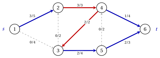
\(\bar{x}_{ij}\)	\(3\)	\(0\)	\(3\)	\(0\)	\(2\)	\(2\)	\(1\)	\(0\)	\(2\)

In the figure each arc carries its capacity \(u_{ij}\).

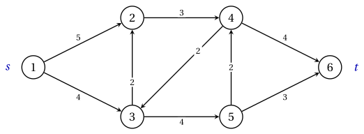
The flow \(\bar{\vet{x}}\) of the table is feasible. For example, at node \(4\) the inflow is \(\bar{x}_{24}+\bar{x}_{54}=3+0=3\) and the outflow is \(\bar{x}_{43}+\bar{x}_{46}=2+1=3\). Its value is

\[ v=\bar{x}_{12}+\bar{x}_{13}=3+0=3 , \]

and node \(6\) receives \(\bar{x}_{46}+\bar{x}_{56}=1+2=3\) units. In the figure each arc carries \(\bar{x}_{ij}/u_{ij}\): the arcs with \(0<\bar{x}_{ij}<u_{ij}\) are blue, the saturated arcs (\(\bar{x}_{ij}=u_{ij}\)) red, and the empty arcs grey and dashed.

5.1.1 The LP model

• We use one continuous variable \(x_{ij}\) for every arc \((i,j) \in A\), the flow on the arc, and one variable \(v\), the value of the flow.

Using these variables, an LP model for the maximum flow problem reads as follows:

\[\begin{align*} && \max \;\; v \label{mf:obj} \tag{5.1a}\\[1ex] && \text{subject to} \quad \sum_{(s,j) \in \delta^+(s)} x_{sj} - \sum_{(j,s) \in \delta^-(s)} x_{js} &= v, & \label{mf:cons-s} \tag{5.1b}\\[1ex] && \sum_{(i,j) \in \delta^+(i)} x_{ij} - \sum_{(j,i) \in \delta^-(i)} x_{ji} &= 0, & \forall i \in N \setminus \{s,t\}, \label{mf:cons} \tag{5.1c}\\[1ex] && \sum_{(t,j) \in \delta^+(t)} x_{tj} - \sum_{(j,t) \in \delta^-(t)} x_{jt} &= -v, & \label{mf:cons-t} \tag{5.1d}\\[1ex] && x_{ij} &\le u_{ij}, & \forall (i,j) \in A, \label{mf:cap} \tag{5.1e}\\[1ex] && x_{ij} &\ge 0, & \forall (i,j) \in A, \label{mf:dom} \tag{5.1f}\\[1ex] && v &\in \R. & \label{mf:domv} \tag{5.1g} \end{align*}\]

This LP model is referred to as the \(\mathrm{MF}\) model.

• Description of the objective function and constraints of the \(\mathrm{MF}\) model:

  • the objective function \(\eqref{mf:obj}\) maximizes the value of the flow;

  • constraint \(\eqref{mf:cons-s}\) states that the net outflow of \(s\) is \(v\), and constraint \(\eqref{mf:cons-t}\) that the net inflow of \(t\) is \(v\);

  • constraints \(\eqref{mf:cons}\) are the flow conservation constraints of the other nodes;

  • constraints \(\eqref{mf:cap}\) impose the capacities, and constraints \(\eqref{mf:dom}\) and \(\eqref{mf:domv}\) define the variables of the LP model.

• Every arc contributes \(+x_{ij}\) to the row of its tail and \(-x_{ij}\) to the row of its head, so the left-hand sides of \(\eqref{mf:cons-s}\)–\(\eqref{mf:cons-t}\) add up to zero: constraint \(\eqref{mf:cons-t}\) follows from the others.

• In Chapter 4, Section «Special cases» the maximum flow problem is a minimum cost flow model: zero balances and zero costs, plus the arc \((t,s)\) with capacity \(+\infty\) and cost \(-1\). Calling \(v\) the flow \(x_{ts}\) on this arc, \(\eqref{mf:cons-s}\)–\(\eqref{mf:cons-t}\) are its conservation constraints, and \(\min\,(-x_{ts})\) is \(\max\, v\).

A feasible flow respects the capacities and is conserved at every node other than \(s\) and \(t\); its value \(v\) is the net outflow of \(s\). The maximum flow problem is the LP \(\mathrm{MF}\): maximize \(v\) under conservation and capacities.

---

Next: 5.2 Cuts