7.4 The potential method

Part 3 · Flows · Chapter 7 · Chapter 7: Transportation and assignment · Lecture notes, volume 3 (PDF) · Exercises: Transportation and assignment

• We write the constraints (7.1c) as \(-\sum_{i \in P} x_{ij}=-d_j\), the conservation constraints of the destinations, and use a free dual variable \(\pi_v\), the potential of node \(v\), for the constraint of every node \(v \in P \cup D\), as in Chapter 4.

Using a free dual variable \(\pi_v\) for the constraint of each node \(v \in P \cup D\), the dual model of the \(\mathrm{TP}\) model is:

\[\begin{align*} && \max \;\;{\sum_{i \in P} a_i \, \pi_i - \sum_{j \in D} d_j \, \pi_j} \label{ta:dobj} \tag{7.2a}\\[1ex] && \text{subject to} \quad \pi_i - \pi_j &\le c_{ij}, & \forall i \in P,~\forall j \in D, \label{ta:dcons} \tag{7.2b}\\[1ex] && \pi_v &\in \R, & \forall v \in P \cup D. \label{ta:dfree} \tag{7.2c} \end{align*}\]

This LP model is referred to as the \(D(\mathrm{TP})\) model.

• With the reduced cost \(\bar{c}_{ij}=c_{ij}-\pi_i+\pi_j\) of Chapter 4, the dual constraint \(\eqref{ta:dcons}\) reads \(\bar{c}_{ij} \ge 0\).

• Adding the same constant to all the potentials changes neither the reduced costs nor, in a balanced instance, the objective \(\eqref{ta:dobj}\). We normalize with \(\pi_{m+n}=0\), the potential of the last destination.

• For every \(\vet{x}\) that satisfies the constraints (7.1b) and (7.1c), the potentials add up row by row and column by column:

  \[ \sum_{i \in P}\sum_{j \in D} (\pi_i-\pi_j)\,x_{ij}=\sum_{i \in P} a_i\,\pi_i-\sum_{j \in D} d_j\,\pi_j , \]

  and since \(c_{ij}=\bar{c}_{ij}+\pi_i-\pi_j\),

  \[ \sum_{i \in P}\sum_{j \in D} c_{ij}\,x_{ij}=\sum_{i \in P}\sum_{j \in D}\bar{c}_{ij}\,x_{ij}+\sum_{i \in P} a_i\,\pi_i-\sum_{j \in D} d_j\,\pi_j . \]

  This is the Lemma «cost and reduced cost» of Chapter 4 for the bipartite network.

Definition 7.9: potentials of a basis

The potentials of a basis \(T\) are the values \(\pi_v\), \(v \in P \cup D\), such that

\[ \bar{c}_{ij}=c_{ij}-\pi_i+\pi_j=0, \quad \forall (i,j) \in T, \qquad\qquad \pi_{m+n}=0 . \]

• The potentials of a basis exist and are unique. Starting from \(\pi_{m+n}=0\), a basic cell \((i,j)\) with one known endpoint gives the other one: \(\pi_i=\pi_j+c_{ij}\) or \(\pi_j=\pi_i-c_{ij}\). Each node is reached along its unique path in the tree from \(m+n\), which forces its value.

Theorem 7.10: optimality criterion

Let \(\bar{\vet{x}}\) be the basic feasible solution of a basis \(T\), with potentials \(\vet{\pi}\). If \(\bar{c}_{ij} \ge 0\) for every cell, then \(\bar{\vet{x}}\) is optimal for the \(\mathrm{TP}\) model, \(\vet{\pi}\) is optimal for the \(D(\mathrm{TP})\) model, and

\[ \sum_{i \in P}\sum_{j \in D} c_{ij}\,\bar{x}_{ij}=\sum_{i \in P} a_i\,\pi_i-\sum_{j \in D} d_j\,\pi_j . \]

If moreover \(\bar{c}_{ij}>0\) for every cell outside \(T\), then \(\bar{\vet{x}}\) is the unique optimal solution.

Proof

We use the identity above. Let \(z_\pi=\sum_{i \in P} a_i\pi_i-\sum_{j \in D} d_j\pi_j\).

1. For \(\bar{\vet{x}}\): \(\bar{c}_{ij}=0\) on \(T\) and \(\bar{x}_{ij}=0\) outside \(T\), so \(\sum \bar{c}_{ij}\bar{x}_{ij}=0\) and the cost of \(\bar{\vet{x}}\) is \(z_\pi\).

2. For every feasible \(\vet{x}\): \(\bar{c} \ge 0\) and \(\vet{x} \ge \vet{0}\), so its cost is at least \(z_\pi\); hence \(\bar{\vet{x}}\) is optimal. The potentials satisfy \(\eqref{ta:dcons}\), and their value \(z_\pi\) equals a primal cost: by weak duality they are optimal.

3. If \(\bar{c}_{ij}>0\) outside \(T\), an optimal \(\vet{x}\) has \(\sum \bar{c}_{ij}x_{ij}=0\), hence \(x_{ij}=0\) outside \(T\): it is the basic solution of \(T\), which is \(\bar{\vet{x}}\) by Theorem 7.6. □

7.4.1 The cycle of a cell and the pivot

Lemma 7.11: the cycle of a non-basic cell

Let \(T\) be a basis and \(e=(k,l) \notin T\). The cells \(T \cup \{e\}\) contain exactly one cycle \(C\), made of \(e\) and of the path from \(l\) to \(k\) in the tree. Write \(C\) starting from \(e\) and moving first along row \(k\), and give the sign \(+\) to the cells in the odd positions (\(e\) included) and \(-\) to the others. Then every row and every column that meets \(C\) contains exactly one cell of \(C\) with sign \(+\) and one with sign \(-\).

Proof

The cycle is the fundamental cycle of the arc \((k,l)\) (Proposition «fundamental cycle» of Chapter 1). It visits the nodes \(k,j_1,i_1,j_2,\dots,l\) alternately in \(P\) and in \(D\), so it has an even number of cells, and two consecutive cells share a node: the first two share the row \(k\), the next two a column, and so on. Every node of \(C\) lies in exactly two cells of \(C\), which are consecutive along \(C\), the last and the first one included: their positions have different parity, hence different signs. □

Theorem 7.12: the pivot

Let \(\bar{\vet{x}}\) be the basic feasible solution of a basis \(T\) with potentials \(\vet{\pi}\), let \(e \notin T\) with \(\bar{c}_e<0\), let \(C^+\) and \(C^-\) be the cells of its cycle with sign \(+\) and \(-\), and let

\[ \theta=\min\{\bar{x}_f : f \in C^-\}, \]

attained at a cell \(f^\ast \in C^-\). For \(0 \le t \le \theta\), let \(\vet{x}(t)\) be \(\bar{\vet{x}}\) with \(t\) added on the cells of \(C^+\) and subtracted on the cells of \(C^-\).

• (a) \(\vet{x}(t)\) is feasible, and its cost is the cost of \(\bar{\vet{x}}\) plus \(t\,\bar{c}_e\).

• (b) \(T'=T \cup \{e\} \setminus \{f^\ast\}\) is a basis, and \(\vet{x}(\theta)\) is its basic feasible solution.

Proof

1. Feasibility. By Lemma 7.11 every row and column of \(C\) gains \(t\) on one cell and loses \(t\) on another, so all the sums are unchanged. The cells of \(C^-\) keep \(\bar{x}_f-t \ge 0\) since \(t \le \theta\).

2. Cost. The change of cost is \(t\big(\sum_{C^+} c_{ij}-\sum_{C^-} c_{ij}\big)\). Every node of \(C\) lies in one cell of \(C^+\) and one of \(C^-\), so \(\sum_{C^+}(\pi_i-\pi_j)=\sum_{C^-}(\pi_i-\pi_j)\), and the change is \(t\big(\sum_{C^+}\bar{c}_{ij}-\sum_{C^-}\bar{c}_{ij}\big)=t\,\bar{c}_e\): the other cells of \(C\) are basic, with \(\bar{c}_{ij}=0\).

3. New basis. \(T'\) has \(m+n-1\) cells, and it has no cycle: the only cycle of \(T \cup \{e\}\) is \(C\), which contains \(f^\ast\). An acyclic set of \(m+n-1\) arcs on \(m+n\) nodes is a spanning tree (Theorem «characterizations of a tree» of Chapter 1). \(\vet{x}(\theta)\) is zero outside \(T'\), since \(x_{f^\ast}(\theta)=0\), so it is the basic solution of \(T'\). □

Algorithm: The potential method

Input: a balanced instance with supplies \(a_i\), demands \(d_j\) and costs \(c_{ij}\)

Output: an optimal basic feasible solution \(\tilde{\vet{x}}\) and optimal potentials \(\tilde{\vet{\pi}}\)

1Step 0 (initial basis). Build a basis \(T\) and its basic feasible solution \(\bar{\vet{x}}\) with the north-west corner rule or the minimum cost rule.

2Step 1 (potentials). Compute the potentials of \(T\) and the reduced costs \(\bar{c}_{ij}=c_{ij}-\pi_i+\pi_j\) of the cells outside \(T\).

3Step 2 (optimality test). If \(\bar{c}_{ij} \ge 0\) for every cell, STOP: \(\bar{\vet{x}}\) is optimal.

4Step 3 (entering cell). Choose a cell \(e\) with \(\bar{c}_e<0\).

5Step 4 (cycle). Find the cycle of \(e\) with its signs, \(\theta:=\min\{\bar{x}_f : f \in C^-\}\), and a leaving cell \(f^\ast \in C^-\) with \(\bar{x}_{f^\ast}=\theta\).

6Step 5 (pivot). Add \(\theta\) on \(C^+\), subtract \(\theta\) on \(C^-\), set \(T:=T \cup \{e\} \setminus \{f^\ast\}\), and go to Step 1.

• Rules of the examples. In Step 3 the entering cell has the most negative reduced cost (the smallest \(i\), then \(j\), on ties). In Step 4 the cycle is written from the entering cell moving first along its row, and the leaving cell is the first cell of \(C^-\) with \(\bar{x}_f=\theta\) in row–column order.

• The method is also known as the u-v method or MODI (modified distribution) method, and the cycle as the stepping stone path: the amounts move along it like on stones across a river.

Theorem 7.13: termination

If \(\theta>0\) at every iteration, the potential method stops after a finite number of iterations with an optimal basic feasible solution and optimal potentials.

Proof

By Theorem 7.12 every iteration with \(\theta>0\) moves to a new basis and decreases the cost by \(\theta\,|\bar{c}_e|>0\). A basis determines its basic solution (Theorem 7.6), so a basis visited twice would have two different costs: no basis repeats. There are finitely many sets of \(m+n-1\) cells, so the method stops, at Step 2, and Theorem 7.10 applies. □

• When \(\theta=0\) the pivot is degenerate: the basis changes, the solution and its cost do not. The potential method is the simplex algorithm on the \(\mathrm{TP}\) model: the basic cells are the basic variables, \(\bar{c}_{ij}\) are their reduced costs, and the cycle describes how the basic variables change when \(x_e\) grows.

• Hence the anti-cycling rule of Bland of Chapter 7 «Optimality conditions and pivot rules» of the module Linear Programming applies: with the first cell with \(\bar{c}_{ij}<0\) in row–column order as the entering cell, and the leaving rule above, no basis repeats even with degenerate pivots.

The u-v convention

Many textbooks write the u-v method with \(u_i+v_j=c_{ij}\) on the basic cells and \(\bar{c}_{ij}=c_{ij}-u_i-v_j\). These are the potentials of this chapter with \(u_i=\pi_i\) for the origins and \(v_j=-\pi_j\) for the destinations: the reduced costs are the same, and the potentials of the destinations change sign.

7.4.2 The potential method on the transportation instance

• We start from the north-west corner solution of Example 7.5, of cost \(440\).

• In each tableau the basic cells (blue) contain the amount \(\bar{x}_{ij}\) in bold, and the other cells the reduced cost \(\bar{c}_{ij}\); the last column and the last row contain the potentials. The entering cell is red, and the cells of the cycle are marked \(\oplus\) and \(\ominus\).

Example 7.7: the potential method from the north-west corner

In the first iteration the potentials of the north-west basis come from \(\pi_7=0\), along the tree:

\[ \pi_2=\pi_7+c_{27}=2,\qquad \pi_3=\pi_7+c_{37}=6,\qquad \pi_5=\pi_2-c_{25}=-2, \]

\[ \pi_6=\pi_2-c_{26}=0,\qquad \pi_1=\pi_5+c_{15}=7,\qquad \pi_4=\pi_1-c_{14}=6 . \]

For example, \(\bar{c}_{35}=c_{35}-\pi_3+\pi_5=1-6-2=-7\).

Iteration 1
	\(4\)	\(5\)	\(6\)	\(7\)	\(\pi_i\)
\(1\)	\(\mathbf{10}\)	\(\mathbf{20}\)	\(-5\)	\(-4\)	\(7\)
\(2\)	\(7\)	\(\mathbf{5}\,\ominus\)	\(\mathbf{15}\)	\(\mathbf{10}\,\oplus\)	\(2\)
\(3\)	\(9\)	\(-7\,\oplus\)	\(-2\)	\(\mathbf{30}\,\ominus\)	\(6\)
\(\pi_j\)	\(6\)	\(-2\)	\(0\)	\(0\)

• The negative reduced costs are \(\bar{c}_{35}=-7\), \(\bar{c}_{16}=-5\), \(\bar{c}_{17}=-4\), \(\bar{c}_{36}=-2\); the cell \((3,5)\) enters the basis.

• The cycle is \(\,(3,5)^{+},\ (3,7)^{-},\ (2,7)^{+},\ (2,5)^{-}\).

• The cells with sign \(-\) have \(\bar{x}_{37}=30\) and \(\bar{x}_{25}=5\): \(\theta=5\), and the cell \((2,5)\) leaves the basis.

• The cost goes from \(440\) to \(440+5\cdot(-7)=405\).

In the network, the entering arc \((3,5)\) (red, dashed) closes the cycle \(3,5,2,7,3\) with the tree.

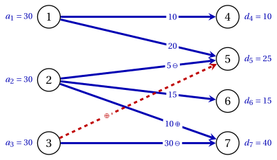
In the second iteration the cycle has six cells and visits all three rows.

Iteration 2
	\(4\)	\(5\)	\(6\)	\(7\)	\(\pi_i\)
\(1\)	\(\mathbf{10}\)	\(\mathbf{20}\,\ominus\)	\(-12\,\oplus\)	\(-11\)	\(14\)
\(2\)	\(14\)	\(7\)	\(\mathbf{15}\,\ominus\)	\(\mathbf{15}\,\oplus\)	\(2\)
\(3\)	\(16\)	\(\mathbf{5}\,\oplus\)	\(-2\)	\(\mathbf{25}\,\ominus\)	\(6\)
\(\pi_j\)	\(13\)	\(5\)	\(0\)	\(0\)

• The negative reduced costs are \(\bar{c}_{16}=-12\), \(\bar{c}_{17}=-11\), \(\bar{c}_{36}=-2\); the cell \((1,6)\) enters the basis.

• The cycle is \(\,(1,6)^{+},\ (1,5)^{-},\ (3,5)^{+},\ (3,7)^{-},\ (2,7)^{+},\ (2,6)^{-}\).

• The cells with sign \(-\) have \(\bar{x}_{15}=20\), \(\bar{x}_{37}=25\) and \(\bar{x}_{26}=15\): \(\theta=15\), and the cell \((2,6)\) leaves the basis.

• The cost goes from \(405\) to \(405+15\cdot(-12)=225\).

Iteration 3
	\(4\)	\(5\)	\(6\)	\(7\)	\(\pi_i\)
\(1\)	\(\mathbf{10}\)	\(\mathbf{5}\,\ominus\)	\(\mathbf{15}\)	\(-11\,\oplus\)	\(14\)
\(2\)	\(14\)	\(7\)	\(12\)	\(\mathbf{30}\)	\(2\)
\(3\)	\(16\)	\(\mathbf{20}\,\oplus\)	\(10\)	\(\mathbf{10}\,\ominus\)	\(6\)
\(\pi_j\)	\(13\)	\(5\)	\(12\)	\(0\)

• The only negative reduced cost is \(\bar{c}_{17}=-11\): the cell \((1,7)\) enters the basis.

• The cycle is \(\,(1,7)^{+},\ (1,5)^{-},\ (3,5)^{+},\ (3,7)^{-}\).

• The cells with sign \(-\) have \(\bar{x}_{15}=5\) and \(\bar{x}_{37}=10\): \(\theta=5\), and the cell \((1,5)\) leaves the basis.

• The cost goes from \(225\) to \(225+5\cdot(-11)=170\).

Iteration 4
	\(4\)	\(5\)	\(6\)	\(7\)	\(\pi_i\)
\(1\)	\(\mathbf{10}\)	\(11\)	\(\mathbf{15}\,\ominus\)	\(\mathbf{5}\,\oplus\)	\(3\)
\(2\)	\(3\)	\(7\)	\(1\)	\(\mathbf{30}\)	\(2\)
\(3\)	\(5\)	\(\mathbf{25}\)	\(-1\,\oplus\)	\(\mathbf{5}\,\ominus\)	\(6\)
\(\pi_j\)	\(2\)	\(5\)	\(1\)	\(0\)

• The only negative reduced cost is \(\bar{c}_{36}=-1\): the cell \((3,6)\) enters the basis.

• The cycle is \(\,(3,6)^{+},\ (3,7)^{-},\ (1,7)^{+},\ (1,6)^{-}\).

• The cells with sign \(-\) have \(\bar{x}_{37}=5\) and \(\bar{x}_{16}=15\): \(\theta=5\), and the cell \((3,7)\) leaves the basis.

• The cost goes from \(170\) to \(170+5\cdot(-1)=165\).

Iteration 5
	\(4\)	\(5\)	\(6\)	\(7\)	\(\pi_i\)
\(1\)	\(\mathbf{10}\)	\(10\)	\(\mathbf{10}\)	\(\mathbf{10}\)	\(3\)
\(2\)	\(3\)	\(6\)	\(1\)	\(\mathbf{30}\)	\(2\)
\(3\)	\(6\)	\(\mathbf{25}\)	\(\mathbf{5}\)	\(1\)	\(5\)
\(\pi_j\)	\(2\)	\(4\)	\(1\)	\(0\)

• All the reduced costs are non-negative: the basic feasible solution is optimal, with cost \(z=165\).

• The optimal solution is

  \[ \tilde{x}_{14}=10,\quad \tilde{x}_{16}=10,\quad \tilde{x}_{17}=10,\quad \tilde{x}_{27}=30,\quad \tilde{x}_{35}=25,\quad \tilde{x}_{36}=5, \qquad z(\mathrm{TP})=165 . \]

  Every cell outside the basis has \(\bar{c}_{ij}>0\), so by Theorem 7.10 the optimum is unique.

• The potentials \(\tilde{\vet{\pi}}=(3,2,5,2,4,1,0)\) are optimal for the \(D(\mathrm{TP})\) model, with value

  \[ 30\,(3+2+5)-(10 \cdot 2+25 \cdot 4+15 \cdot 1+40 \cdot 0)=300-135=165 . \]

  Gurobi returns the same optimal solution, and its dual values coincide with \(\tilde{\vet{\pi}}\).

• From the minimum cost solution of Example 7.6 the method needs a single pivot: that solution has the basis of iteration \(4\), and the entering cell \((3,6)\), with \(\theta=5\), gives the optimum.

7.4.3 Degeneracy

Example 7.8: a degenerate pivot

We consider the instance

\[ \begin{array}{c|ccc|c} \hline {c_{ij}} & {4} & {5} & {6} & {a_i} \\ \hline {1} & {1} & {4} & {7} & {30} \\ {2} & {6} & {2} & {5} & {25} \\ {3} & {3} & {9} & {5} & {30} \\ \hline {d_j} & {30} & {30} & {25} & {85} \\ \hline \end{array} \]

• In the north-west corner rule the first cell exhausts row \(1\) and column \(4\) at once. Only the row is crossed out, and the cell \((2,4)\) enters \(T\) with the amount \(0\): the solution, of cost \(250\), is degenerate.

step	cell	amount	crossed out
\(1\)	\((1,4)\)	\(30\)	row \(1\)
\(2\)	\((2,4)\)	\(0\)	column \(4\)
\(3\)	\((2,5)\)	\(25\)	row \(2\)
\(4\)	\((3,5)\)	\(5\)	column \(5\)
\(5\)	\((3,6)\)	\(25\)	row \(3\), column \(6\)

Iteration 1
	\(4\)	\(5\)	\(6\)	\(\pi_i\)
\(1\)	\(\mathbf{30}\)	\(7\)	\(14\)	\(-7\)
\(2\)	\(\mathbf{0}\,\ominus\)	\(\mathbf{25}\,\oplus\)	\(7\)	\(-2\)
\(3\)	\(-10\,\oplus\)	\(\mathbf{5}\,\ominus\)	\(\mathbf{25}\)	\(5\)
\(\pi_j\)	\(-8\)	\(-4\)	\(0\)

• The only negative reduced cost is \(\bar{c}_{34}=-10\): the cell \((3,4)\) enters the basis.

• The cycle is \(\,(3,4)^{+},\ (3,5)^{-},\ (2,5)^{+},\ (2,4)^{-}\).

• The cells with sign \(-\) have \(\bar{x}_{35}=5\) and \(\bar{x}_{24}=0\): \(\theta=0\), and the cell \((2,4)\) leaves the basis.

• The pivot is degenerate: the solution and its cost \(z=250\) do not change, only the basis does.

In the second iteration the basis has changed, so the potentials have changed too: now \(\bar{c}_{15}<0\).

Iteration 2
	\(4\)	\(5\)	\(6\)	\(\pi_i\)
\(1\)	\(\mathbf{30}\,\ominus\)	\(-3\,\oplus\)	\(4\)	\(3\)
\(2\)	\(10\)	\(\mathbf{25}\)	\(7\)	\(-2\)
\(3\)	\(\mathbf{0}\,\oplus\)	\(\mathbf{5}\,\ominus\)	\(\mathbf{25}\)	\(5\)
\(\pi_j\)	\(2\)	\(-4\)	\(0\)

• The only negative reduced cost is \(\bar{c}_{15}=-3\): the cell \((1,5)\) enters the basis.

• The cycle is \(\,(1,5)^{+},\ (1,4)^{-},\ (3,4)^{+},\ (3,5)^{-}\).

• The cells with sign \(-\) have \(\bar{x}_{14}=30\) and \(\bar{x}_{35}=5\): \(\theta=5\), and the cell \((3,5)\) leaves the basis.

• The cost goes from \(250\) to \(250+5\cdot(-3)=235\).

Iteration 3
	\(4\)	\(5\)	\(6\)	\(\pi_i\)
\(1\)	\(\mathbf{25}\)	\(\mathbf{5}\)	\(4\)	\(3\)
\(2\)	\(7\)	\(\mathbf{25}\)	\(4\)	\(1\)
\(3\)	\(\mathbf{5}\)	\(3\)	\(\mathbf{25}\)	\(5\)
\(\pi_j\)	\(2\)	\(-1\)	\(0\)

• All the reduced costs are non-negative: the basic feasible solution is optimal, with cost \(z=235\).

The optimal solution is unique, with cost \(235\), and Gurobi confirms it.

• The basic cell with value \(0\) must be kept in \(T\): without it, the other four cells would not span the six nodes, and the potentials could not be computed.

• The degenerate pivot of iteration \(1\) does not lower the cost, but it moves to a basis whose potentials reveal an improving cell.

The potential method computes the potentials of the basis (\(\bar{c}_{ij}=0\) on the basic cells, \(\pi_{m+n}=0\)), stops when every reduced cost is non-negative, and otherwise moves \(\theta\) units around the cycle of an entering cell. The cost decreases by \(\theta\,|\bar{c}_e|\); with \(\theta=0\) only the basis changes.

---

Next: 7.5 The assignment problem