4.9 A transshipment instance

Part 3 · Flows · Chapter 4 · Chapter 4: Flow models · Lecture notes, volume 3 (PDF) · Exercises: Flow models

- We solve the \(\mathrm{MCF}\) model of Example 4.2: the reference network, with two supply nodes, two demand nodes and two transshipment nodes. The optimal solution is computed with Gurobi (gurobipy), and then certified by hand with Corollary 4.20.

Example 4.9: the optimal flow

The optimal flow \(\tilde{\vet{x}}\) and its optimal value are

arc	\((1,2)\)	\((1,3)\)	\((2,4)\)	\((3,2)\)	\((3,5)\)	\((4,3)\)	\((4,6)\)	\((5,4)\)	\((5,6)\)
\(\tilde{x}_{ij}\)	\(2\)	\(3\)	\(4\)	\(0\)	\(3\)	\(0\)	\(2\)	\(1\)	\(2\)
\(u_{ij}\)	\(4\)	\(4\)	\(4\)	\(2\)	\(4\)	\(3\)	\(5\)	\(3\)	\(2\)

\(z(\mathrm{MCF})=60\).

In the figure each arc carries \(\tilde{x}_{ij}/u_{ij}\): the arcs strictly between their bounds are blue, the arcs at capacity red, the empty arcs grey and dashed. Next to each node, its potential.

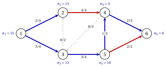
The flow is integer, as Corollary 4.16 guarantees.

4.9.1 The certificate of optimality

1. The five blue arcs \((1,2)\), \((1,3)\), \((3,5)\), \((4,6)\), \((5,4)\) form a spanning tree. We ask for reduced cost zero on them, \(\pi_i-\pi_j=c_{ij}\), and normalize with \(\pi_6=0\).

2. Going backwards from node \(6\): \(\pi_4=\pi_6+c_{46}=5\), \(\pi_5=\pi_4+c_{54}=10\), \(\pi_3=\pi_5+c_{35}=13\), \(\pi_1=\pi_3+c_{13}=15\) and \(\pi_2=\pi_1-c_{12}=13\).

3. The potential \(\pi_i\) is the cost of the tree path from \(i\) to \(6\): for example, \(\pi_1=c_{13}+c_{35}+c_{54}+ c_{46}=2+3+5+5=15\).

Example 4.10: reduced costs and optimality

The reduced costs \(\bar{c}_{ij}=c_{ij}-\pi_i+\pi_j\) are:

arc	\((1,2)\)	\((1,3)\)	\((2,4)\)	\((3,2)\)	\((3,5)\)	\((4,3)\)	\((4,6)\)	\((5,4)\)	\((5,6)\)
\(\bar{c}_{ij}\)	\(0\)	\(0\)	\(-3\)	\(2\)	\(0\)	\(11\)	\(0\)	\(0\)	\(-7\)
\(\alpha_{ij}\)	\(0\)	\(0\)	\(3\)	\(0\)	\(0\)	\(0\)	\(0\)	\(0\)	\(7\)

• The arcs with \(\bar{c}_{ij}>0\), \((3,2)\) and \((4,3)\), are empty; the arcs with \(\bar{c}_{ij}<0\), \((2,4)\) and \((5,6)\), are at capacity. By Corollary 4.20, \(\tilde{\vet{x}}\) is optimal.

• The dual value is \(\sum_{i \in N} b_i\pi_i-\sum_{(i,j) \in A} u_{ij}\alpha_{ij}=86-26=60\), equal to the cost of \(\tilde{\vet{x}}\). The potentials coincide with the dual values returned by Gurobi, shifted so that \(\pi_6=0\).

• Uniqueness. Every optimal flow has gap zero with \((\vet{\pi},\vet{\alpha})\), so by Theorem 4.19 it has \(x_{32}=x_{43}=0\), \(x_{24}=4\) and \(x_{56}=2\). The flow on the five tree arcs is then fixed by conservation, since their columns are linearly independent: \(\tilde{\vet{x}}\) is the unique optimal flow.

• The flow \(\bar{\vet{x}}\). The feasible flow \(\bar{\vet{x}}\) of Example 4.1 costs \(63\), and its gap with the same dual solution is \(63-60=3=\alpha_{24}(u_{24}-\bar{x}_{24})=3 \cdot (4-3)\): the arc \((2,4)\) is not used enough.

On the reference network the optimal flow costs \(60\). The potentials of its spanning tree give reduced costs that are positive only on empty arcs and negative only on saturated arcs: they certify the optimality without a solver.

4.10 Typical mistakes

Warning

• Swapping outflow and inflow. The conservation constraint is outflow minus inflow equal to \(b_i\), with \(b_i>0\) at a supply node: the signs follow the incidence matrix, \(+1\) in the tail.

• Taking \(\sum_i b_i=0\) as sufficient. A balanced network can have no feasible flow: a cut may be too small to carry the supply inside it.

• Getting the substitution signs wrong. With \(\vet{x}=\vet{l}+\vet{x}'\) the tail of \((i,j)\) loses \(l_{ij}\) units of balance and the head gains them; the constant \(\vet{c}'\vet{l}\) must be added back to the value.

• Forgetting the dummy node. An instance with more supply than demand has no feasible flow with equalities; the dummy arcs must cost zero, or the unused supply is charged.

• Claiming integrality for any matrix. Integer vertices need a TU matrix and integer \(\vet{b}\), \(\vet{l}\), \(\vet{u}\); the costs may be fractional.

• Writing the reduced cost with the wrong signs. In this module \(\bar{c}_{ij}=c_{ij}-\pi_i+\pi_j\), with \(-\pi\) of the tail and \(+\pi\) of the head.

• Expecting unique potentials. The potentials are defined up to an additive constant; they are fixed by a normalization such as \(\pi_n=0\).

4.11 In summary

In summary

• A network has balances \(b_i\), lower bounds \(l_{ij}\), capacities \(u_{ij}\) and costs \(c_{ij}\); the minimum cost flow problem is the LP \(\min\{\vet{c}'\vet{x} : \mat{B}\vet{x}=\vet{b},~\vet{l} \le \vet{x} \le \vet{u}\}\).

• Across every cut the net outflow equals the balance inside; a feasible network is balanced and satisfies the cut condition.

• Lower bounds are removed with \(\vet{x}=\vet{l}+\vet{x}'\); an excess of supply goes to a dummy node through zero-cost arcs.

• The incidence matrix is totally unimodular, so with integer \(\vet{b}\), \(\vet{l}\), \(\vet{u}\) every vertex is integer and the \(\mathrm{MCF}\) model has an integer optimal solution.

• The dual has potentials \(\pi_i\); with \(\bar{c}_{ij}=c_{ij}-\pi_i+\pi_j\), a flow with empty positive-cost arcs and saturated negative-cost arcs is optimal.

• Shortest path, maximum flow, transportation and assignment are \(\mathrm{MCF}\) models.

The reference network at a glance.

balances	\(\vet{b}=(5,2,0,-3,0,-4)\)
optimal flow	\(\tilde{\vet{x}}=(2,3,4,0,3,0,2,1,2)\), \(z(\mathrm{MCF})=60\)
potentials (\(\pi_6=0\))	\(\vet{\pi}=(15,13,13,5,10,0)\)
empty / saturated arcs	\((3,2)\), \((4,3)\) / \((2,4)\), \((5,6)\)
with \(l_{32}=1\)	\(\vet{b}'=(5,3,-1,-3,0,-4)\), optimal value \(62\)
with \(b_2=4\) (dummy node \(7\))	\(x_{17}=2\), optimal value \(56\)

---

Exercises on this chapter: Flow models