Phase 0 of the simplex algorithm¶

Part 2 · The simplex algorithm · Chapter 8 · Lecture notes, volume 2 (PDF) · Exercises: Phase 0 of the simplex algorithm

8.1 The simplex auxiliary problem¶

We consider an LP problem in standard maximization form with \(n+m\) non-negative variables and \(m\) equality linear constraints, obtained from an LP problem in canonical maximization form with \(n\) non-negative variables and \(m\) less-than-or-equal-to linear constraints by adding \(m\) slack non-negative variables:

\[\begin{align*} && \max \;\;{\boldsymbol c}' \, {\boldsymbol x} \label{FORM_STANDARD_OBJ} \tag{8.1a}\\[2ex] && \text{subject to} \quad {\boldsymbol A} \; {\boldsymbol x} &= {\boldsymbol b}, & \phantom{j=1111} \label{FORM_STANDARD_CONS1} \tag{8.1b}\\[2ex] && {\boldsymbol x} &\ge {\boldsymbol 0}. \label{FORM_STANDARD_CONS2} \tag{8.1c} \end{align*}\]
The Step \(0\) of the simplex algorithm requires an initial basic feasible solution. If \({\boldsymbol b} \ge {\boldsymbol 0}\), the partition

\[ \pazocal{B}=\{n+1,n+2,\dots,n+m\} \text{ and } \pazocal{N}=\{1,2,\dots,n\} \]

is associated with the basis \({\boldsymbol A}_{\pazocal{B}} = {\boldsymbol I}\) and with the initial basic feasible solution \({\boldsymbol x}_{\pazocal{B}} = {\boldsymbol b}\) and \({\boldsymbol x}_{\pazocal{N}} = {\boldsymbol 0}\).
If instead \(b_i < 0\) for some \(i \in \{1,2,\dots,m\}\), this partition is not associated with a basic feasible solution, and the simplex algorithm cannot be started. In this case we execute the Phase \(0\) of the simplex algorithm.

Definition 8.1: Phase \(0\) of the simplex algorithm

The Phase \(0\) of the simplex algorithm is a procedure which determines a basic feasible solution of the LP problem (8.1), together with the associated dictionary, or proves that the LP problem (8.1) is infeasible.

Definition 8.2: simplex auxiliary problem

Given an LP problem (8.1) in standard maximization form, the associated simplex auxiliary problem is the LP problem in standard maximization form obtained by adding one non-negative variable \(x_0\), called the auxiliary variable, subtracting it from the left-hand side of every linear constraint, and replacing the objective function:

\[\begin{align*} \label{OBJ_AUX} && \max \;\; - \; x_0 \tag{8.2a}\\[1.5ex] \label{CONS1_AUX} && \text{subject to} \quad \sum_{j=1}^{n+m} \; {a_{ij} \; x_j} - x_0 & = b_i, & \forall \;\; i \in \{1,2,\dots,m\} \tag{8.2b}\\[1.5ex] \label{CONS2_AUX} && x_0, \; x_j &\ge 0, & \forall \;\; j \in \{1,2,\dots,n+m\} \tag{8.2c} \end{align*}\]

The auxiliary variable \(x_0\) is placed in the first position, and then the input data of the simplex auxiliary problem (8.2) are the column vector \({\boldsymbol x} \in \R^{n+m+1}\) of the variables, the objective-function vector \({\boldsymbol c} \in \Z^{n+m+1}\), whose first entry is \(-1\) and whose other entries are \(0\), the constraint matrix \({\boldsymbol A} \in \Z^{m \times (n+m+1)}\), obtained by prepending to the original constraint matrix a column of \(m\) entries all equal to \(-1\), and the right-hand-side vector \({\boldsymbol b} \in \Z^{m}\):

\[ {\boldsymbol x}= \begin{pmatrix} x_{0} \\ x_{1} \\ \vdots \\ x_{n} \\[1ex] x_{n+1} \\ \vdots \\ x_{n+m} \\ \end{pmatrix} \quad {\boldsymbol c}= \begin{pmatrix} -1\\ 0\\ \vdots\\ \vdots \\[1ex] \vdots\\ \vdots\\ 0\\ \end{pmatrix} \quad {\boldsymbol A}= \begin{pmatrix} -1 & a_{11} & \dots & a_{1n} &1& \dots&0\\ -1 & a_{21} & \dots & a_{2n}&0& \dots&0\\ \vdots & \vdots & \dots & \vdots &\vdots& \dots&\vdots\\ -1 & a_{m1} & \dots & a_{mn}&0& \dots&1\\ \end{pmatrix} \quad {\boldsymbol b}= \begin{pmatrix} b_{1} \\ b_{2} \\ \vdots \\ b_{m} \\ \end{pmatrix} \]

The simplex auxiliary problem (8.2) is never infeasible and it is never unbounded:

it always admits a feasible solution, obtained by setting \(x_j = 0\) for every \(j \in \{1,2,\dots,n\}\), \(x_0 = \max\{0, -\min_{i} b_i\}\) and the slack variables \(x_{n+i} = b_i + x_0 \ge 0\) for every \(i \in \{1,2,\dots,m\}\);
its objective value is \(-x_0 \le 0\) for every feasible solution.

Accordingly, by the Fundamental Theorem of Linear Programming, it always admits an optimal solution.

Theorem 8.3: feasibility of an LP problem

The LP problem (8.1) admits a feasible solution if and only if the optimal value of the associated simplex auxiliary problem (8.2) is equal to \(0\).

The idea of the proof is that a feasible solution of the LP problem (8.1) is exactly a feasible solution of the simplex auxiliary problem (8.2) in which the auxiliary variable takes the value \(x_0 = 0\).

Proof

We prove the two implications separately.

\((\Rightarrow)\) Let \(\bar{\boldsymbol x}\) be a feasible solution of the LP problem (8.1). The point obtained by adding \(\bar x_0 = 0\) is a feasible solution of the simplex auxiliary problem (8.2), since

\[ \sum_{j=1}^{n+m} a_{ij} \, \bar x_j - \underbrace{\bar x_0}_{=0} = b_i, \qquad \forall i \in \{1,2,\dots,m\}, \]

and its objective value is \(-\bar x_0 = 0\). Since the objective value of every feasible solution of (8.2) is \(-x_0 \le 0\), this solution is optimal and the optimal value is \(0\).

\((\Leftarrow)\) Let the optimal value of the simplex auxiliary problem (8.2) be equal to \(0\) and let \(\tilde{\boldsymbol x}\) be an optimal solution. Then \(\tilde x_0 = 0\) and, by \(\eqref{CONS1_AUX}\),

\[ \sum_{j=1}^{n+m} a_{ij} \, \tilde x_j = b_i + \underbrace{\tilde x_0}_{=0} = b_i, \qquad \forall i \in \{1,2,\dots,m\} . \]

Accordingly, the point obtained by removing the auxiliary variable satisfies the equality constraints \(\eqref{FORM_STANDARD_CONS1}\) and the non-negativity constraints \(\eqref{FORM_STANDARD_CONS2}\), and then it is a feasible solution of the LP problem (8.1). □

If the optimal value of the simplex auxiliary problem (8.2) is strictly negative, then the LP problem (8.1) is infeasible.

Example 8.1: simplex auxiliary problem

Consider the following LP problem in canonical maximization form with \(n=2\) non-negative variables and \(m=3\) less-than-or-equal-to linear constraints (called Example 8.1):

\[ \begin{array}{rrrrrrrrrrrrr} {\max} & \, {x_1} & {+} & {2} \, {x_2} \\[1ex] \text{subject to} & {-} \, {x_1} & {-} & \, {x_2} & {\le} & {-3} \\[1ex] & {-} \, {x_1} & {+} & \, {x_2} & {\le} & {2} \\[1ex] & \, {x_1} & {+} & \, {x_2} & {\le} & {6} \\[1ex] & {x_1,} & & {x_2} & { \ge} & {0} \end{array} \]

By adding \(m=3\) slack variables, we obtain the following LP problem in standard maximization form with \(n+m=5\) non-negative variables:

\[ \begin{array}{rrrrrrrrrrrrrrrrrrr} {\max} & \, {x_1} & {+} & {2} \, {x_2} & & \\[1ex] \text{subject to} & {-x_1} & {-} & \, {x_2} & {+} \, {x_3} & & & {=} & {-3} \\[1ex] & {-x_1} & {+} & \, {x_2} & & {+} \, {x_4} & & {=} & {2} \\[1ex] & {x_1} & {+} & \, {x_2} & & & {+} \, {x_5} & {=} & {6} \\[1ex] & {x_1,} & & {x_2,} & \, {x_3,} & \, {x_4,} & \, {x_5} & { \ge} & { 0 } \end{array} \]

Since \(b_1 = -3 < 0\), the partition \(\pazocal{B}= \{3,~~4,~~5\}\) and \(\pazocal{N}= \{1,~~2\}\) is not associated with a basic feasible solution, and we have to execute the Phase \(0\).

The associated simplex auxiliary problem with \(n+m+1=6\) non-negative variables reads as follows:

\[ \begin{array}{rrrrrrrrrrrrrrrrrrr} {\max} & {-} \, {x_0} & & & & \\[1ex] \text{subject to} & {-} \, {x_0} & {-} & \, {x_1} & {-} & \, {x_2} & {+} \, {x_3} & & & {=} & {-3} \\[1ex] & {-} \, {x_0} & {-} & \, {x_1} & {+} & \, {x_2} & & {+} \, {x_4} & & {=} & {2} \\[1ex] & {-} \, {x_0} & {+} & \, {x_1} & {+} & \, {x_2} & & & {+} \, {x_5} & {=} & {6} \\[1ex] & {x_0,} & & {x_1,} & & {x_2,} & \, {x_3,} & \, {x_4,} & \, {x_5} & { \ge} & { 0 } \end{array} \]

8.2 Solving the simplex auxiliary problem¶

The simplex auxiliary problem (8.2) is solved with the simplex algorithm. Its \(m\) slack variables give the partition

\[ \pazocal{B}=\{n+1,n+2,\dots,n+m\} \text{ and } \pazocal{N}=\{0,1,2,\dots,n\}, \]

which is associated with the basis \({\boldsymbol A}_{\pazocal{B}} = {\boldsymbol I}\) and with the dictionary

\[\begin{equation*} \begin{cases} \displaystyle x_{i} = {{ b_i}} - \sum_{j \in \pazocal{N}} \bar{a}_{ij} \; x_{j},~~ \forall i \in \pazocal{B}\\[4ex] \displaystyle - w = 0 - x_{0}, \end{cases} \end{equation*}\]

where \(-w = -x_0\) denotes the objective function of the simplex auxiliary problem (i.e., \(w = x_0\)). This dictionary is not associated with a basic feasible solution, since \(b_i < 0\) for some \(i \in \pazocal{B}\).
A single special pivoting operation is enough to obtain a basic feasible solution of the simplex auxiliary problem: the auxiliary variable \(x_0\) enters the basis, and the basic variable leaving the basis is the one with the most negative value.

Special pivoting operation. The pivot column is the auxiliary variable \(x_0\) and the pivot row is the basic variable \(x_r\) with

\[ r \in \argmin \{\, b_i : i \in \pazocal{B} \,\} . \]

After this pivoting operation, the values of the variables are

\[ x_0 = - b_r \qquad \text{and} \qquad x_i = b_i - b_r, \quad \forall i \in \pazocal{B} \setminus \{r\} , \]

and they are all non-negative, since \(b_r \le b_i\) for every \(i \in \pazocal{B}\).

Starting from the basic feasible solution obtained with the special pivoting operation, the simplex algorithm is executed on the simplex auxiliary problem until an optimal solution is found. Since the simplex auxiliary problem is never unbounded, the algorithm always terminates with an optimal dictionary.

At the end of the Phase \(0\), exactly one of the following three cases occurs:

the optimal value of the simplex auxiliary problem is strictly negative: the LP problem (8.1) is infeasible;
the optimal value is \(0\) and the auxiliary variable \(x_0\) is non-basic: the optimal basis of the simplex auxiliary problem, after removing \(x_0\) from \(\pazocal{N}\), is a basis of the LP problem (8.1) associated with a basic feasible solution;
the optimal value is \(0\) and the auxiliary variable \(x_0\) is basic, necessarily with value \(x_0 = 0\): one further pivoting operation makes \(x_0\) leave the basis, bringing back to the previous case.

In the third case, the basic feasible solution of the simplex auxiliary problem is degenerate, since the basic variable \(x_0\) takes the value \(0\). A pivoting operation is performed on the row of \(x_0\), choosing as pivot column any non-basic variable \(x_j\) with \(j \in \pazocal{N}\) such that \(\bar{a}_{0j} \ne 0\): the value of the other basic variables does not change, since the value of \(x_0\) is \(0\). Such a variable always exists: otherwise, the row of \(x_0\) in \({\boldsymbol A}_{\pazocal{B}}^{-1}{\boldsymbol A}\) (without the column of \(x_0\)) would be zero, contradicting \(\rank({\boldsymbol A}) = m\), which holds since \({\boldsymbol A}\) contains the identity matrix of the slack variables.

Example 8.2: Phase \(0\) of the simplex algorithm

Consider the simplex auxiliary problem of Example 8.1. With \(\pazocal{B}= \{3,~~4,~~5\}\) and \(\pazocal{N}= \{0,~~1,~~2\}\), the initial dictionary is:

\[\begin{equation*} \begin{cases} \begin{array}{rrrrrrrrrrrrr} {x_3} & {=} & {-3} & {+} & {x_0} & {+} & {x_1} & {+} & {x_2} \\[2ex] {x_4} & {=} & {2} & {+} & {x_0} & {+} & {x_1} & {-} & {x_2} \\[2ex] {x_5} & {=} & {6} & {+} & {x_0} & {-} & {x_1} & {-} & {x_2} \\[2ex] {-w} & {=} & {0} & {-} & {x_0} & & & & \end{array} \end{cases} \end{equation*}\]

The associated basic solution is not feasible, since \(\bar b_3 = -3 < 0\).

Special pivoting operation. The pivot column is \(x_0\) and the pivot row is \(x_3\), the basic variable with the most negative value. By isolating \(x_0\) in the first equation we obtain \(x_0 = 3 + x_3 - x_1 - x_2\), and by substituting it in the other equations we obtain the dictionary with \(\pazocal{B}= \{0,~~4,~~5\}\) and \(\pazocal{N}= \{1,~~2,~~3\}\):

\[\begin{equation*} \begin{cases} \begin{array}{rrrrrrrrrrrrr} {x_0} & {=} & {3} & {-} & {x_1} & {-} & {x_2} & {+} & {x_3} \\[2ex] {x_4} & {=} & {5} & & & {-} & {2\,x_2} & {+} & {x_3} \\[2ex] {x_5} & {=} & {9} & {-} & {2\,x_1} & {-} & {2\,x_2} & {+} & {x_3} \\[2ex] {-w} & {=} & {-3} & {+} & {x_1} & {+} & {x_2} & {-} & {x_3} \end{array} \end{cases} \end{equation*}\]

The associated basic feasible solution is \(\bar x_0 = 3\), \(\bar x_4 = 5\), \(\bar x_5 = 9\) and \(\bar x_1 = \bar x_2 = \bar x_3 = 0\), of value \(-w = -3\).

First pivoting operation. The reduced cost of \(x_1\) is \(\bar c_1 = 1 > 0\), and then the pivot column is \(x_1\). The values of its column are \(\bar a_{01} = 1\) and \(\bar a_{51} = 2\), and then

\[ t_m = \min \left\{~\frac{3}{1},~\frac{9}{2}~\right\} = 3 \]

and the pivot row is \(x_0\). The new dictionary, with \(\pazocal{B}= \{1,~~4,~~5\}\) and \(\pazocal{N}= \{0,~~2,~~3\}\), is:

\[\begin{equation*} \begin{cases} \begin{array}{rrrrrrrrrrrrr} {x_1} & {=} & {3} & {-} & {x_0} & {-} & {x_2} & {+} & {x_3} \\[2ex] {x_4} & {=} & {5} & & & {-} & {2\,x_2} & {+} & {x_3} \\[2ex] {x_5} & {=} & {3} & {+} & {2\,x_0} & & & {-} & {x_3} \\[2ex] {-w} & {=} & {0} & {-} & {x_0} & & & & \end{array} \end{cases} \end{equation*}\]

All the reduced costs are non-positive, and then this dictionary is optimal: the optimal value of the simplex auxiliary problem is \(0\) and the auxiliary variable \(x_0\) is non-basic. Accordingly, the LP problem of Example 8.1 is feasible and

\[ \pazocal{B}= \{1,~~4,~~5\} \]

is a basis associated with a basic feasible solution.

8.3 From the Phase \(0\) to the simplex algorithm¶

At the end of the Phase \(0\), the optimal dictionary of the simplex auxiliary problem gives the equations of the basic variables of the LP problem (8.1) in function of its non-basic variables, once the auxiliary variable \(x_0\) is removed from \(\pazocal{N}\).
The last equation of that dictionary, however, is the one of the objective function \(-w\) of the simplex auxiliary problem, and it has to be replaced by the equation of the original objective function \(z\).

The equation of the original objective function is obtained by substituting, in

\[ z = \sum_{j=1}^{n+m} c_j \; x_j , \]

the equation of every basic variable \(x_i\) with \(i \in \pazocal{B}\), so that \(z\) is written in function of the non-basic variables only. Equivalently, it is computed as

\[ \bar{z} = {\boldsymbol c}'_{\pazocal{B}} \; {\boldsymbol A}_{\pazocal{B}}^{-1} \; {\boldsymbol b} \qquad \text{and} \qquad {{ \bar{\boldsymbol c}}'} = {\boldsymbol c}'_{\pazocal{N}} - {\boldsymbol c}'_{\pazocal{B}} \; {\boldsymbol A}_{\pazocal{B}}^{-1} \;{\boldsymbol A}_{\pazocal{N}} . \]

Once the initial dictionary of the LP problem (8.1) is available, the simplex algorithm is executed as usual, starting from its Step \(1\).

Example 8.3: from the Phase \(0\) to the simplex algorithm

Consider the optimal dictionary of the simplex auxiliary problem of Example 8.1, with \(\pazocal{B}= \{1,~~4,~~5\}\). By removing the auxiliary variable \(x_0\), the equations of the basic variables of the LP problem are:

\[ \begin{cases} x_1 = 3 - x_2 + x_3\\[1ex] x_4 = 5 - 2\,x_2 + x_3\\[1ex] x_5 = 3 - x_3 \end{cases} \]

The objective function of the LP problem of Example 8.1 is \(z = x_1 + 2 \, x_2\), and the basic variable \(x_1\) appears in it. By substituting its equation, we obtain:

\[ z = \underbrace{3 - x_2 + x_3}_{= \, x_1} + 2 \, x_2 = 3 + x_2 + x_3 . \]

Accordingly, with \(\pazocal{B}= \{1,~~4,~~5\}\) and \(\pazocal{N}= \{2,~~3\}\), the initial dictionary of the LP problem of Example 8.1 is:

\[\begin{equation*} \begin{cases} \begin{array}{rrrrrrrrrrrrr} {x_1} & {=} & {3} & {-} & {x_2} & {+} & {x_3} \\[2ex] {x_4} & {=} & {5} & {-} & {2\,x_2} & {+} & {x_3} \\[2ex] {x_5} & {=} & {3} & & & {-} & {x_3} \\[2ex] {z} & {=} & {3} & {+} & {x_2} & {+} & {x_3} \end{array} \end{cases} \end{equation*}\]

and the associated basic feasible solution is \(\bar x_1 = 3\), \(\bar x_4 = 5\), \(\bar x_5 = 3\) and \(\bar x_2 = \bar x_3 = 0\), of value \(3\).

Example 8.4: execution of the simplex algorithm after the Phase \(0\)

Starting from the initial dictionary of Example 8.1 determined by the Phase \(0\), we execute the simplex algorithm.

First pivoting operation. The reduced cost of \(x_2\) is \(\bar c_2 = 1 > 0\), and then the pivot column is \(x_2\). The values of its column are \(\bar a_{12} = 1\) and \(\bar a_{42} = 2\), and then

\[ t_m = \min \left\{~\frac{3}{1},~\frac{5}{2}~\right\} = \frac{5}{2} \]

and the pivot row is \(x_4\). The new dictionary, with \(\pazocal{B}= \{1,~~2,~~5\}\) and \(\pazocal{N}= \{3,~~4\}\), is:

\[\begin{equation*} \begin{cases} \begin{array}{rrrrrrrrrrrrr} {x_1} & {=} & {\frac{1}{2}} & {+} & {\frac{1}{2}\,x_3} & {+} & {\frac{1}{2}\,x_4} \\[2ex] {x_2} & {=} & {\frac{5}{2}} & {+} & {\frac{1}{2}\,x_3} & {-} & {\frac{1}{2}\,x_4} \\[2ex] {x_5} & {=} & {3} & {-} & {x_3} & & \\[2ex] {z} & {=} & {\frac{11}{2}} & {+} & {\frac{3}{2}\,x_3} & {-} & {\frac{1}{2}\,x_4} \end{array} \end{cases} \end{equation*}\]

Second pivoting operation. The reduced cost of \(x_3\) is \(\bar c_3 = \frac{3}{2} > 0\), and then the pivot column is \(x_3\). The only positive value in its column is \(\bar a_{53} = 1\), and then \(t_m = \frac{3}{1} = 3\) and the pivot row is \(x_5\). The new dictionary, with \(\pazocal{B}= \{1,~~2,~~3\}\) and \(\pazocal{N}= \{4,~~5\}\), is:

\[\begin{equation*} \begin{cases} \begin{array}{rrrrrrrrrrrrr} {x_1} & {=} & {2} & {+} & {\frac{1}{2}\,x_4} & {-} & {\frac{1}{2}\,x_5} \\[2ex] {x_2} & {=} & {4} & {-} & {\frac{1}{2}\,x_4} & {-} & {\frac{1}{2}\,x_5} \\[2ex] {x_3} & {=} & {3} & & & {-} & {x_5} \\[2ex] {z} & {=} & {10} & {-} & {\frac{1}{2}\,x_4} & {-} & {\frac{3}{2}\,x_5} \end{array} \end{cases} \end{equation*}\]

All the reduced costs are non-positive, and then this dictionary is optimal. An optimal solution of the LP problem of Example 8.1 is

\[ \tilde{\boldsymbol x}(\, LP \,) = \begin{pmatrix} 2 \\[0.5ex] 4 \end{pmatrix} \]

and the optimal value is \(z(\, LP \,) = 10\).

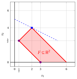
The feasible region \(F\) is bounded by the lines \(-x_1 - x_2 = -3\) (bottom left), \(-x_1 + x_2 = 2\) (top left), \(x_1 + x_2 = 6\) (right) and the \(x_1\)-axis; in dashed blue the level set \(x_1 + 2\,x_2 = 10\) through the optimal vertex. In violet the basic feasible solution \((3,0)\) determined by the Phase \(0\) and the vertex \((\frac{1}{2},\frac{5}{2})\) reached after the first pivoting operation, in blue the optimal solution reached by the simplex algorithm.

8.4 Detecting infeasible LP problems¶

If the optimal value of the simplex auxiliary problem (8.2) is strictly negative, then, by Theorem 8.3, the LP problem (8.1) is infeasible. In this case the optimal dictionary of the simplex auxiliary problem is a certificate of infeasibility.

Example 8.5: infeasible LP problem

Consider the following LP problem in canonical maximization form with \(n=2\) non-negative variables and \(m=2\) less-than-or-equal-to linear constraints (called Example 8.5):

\[ \begin{array}{rrrrrrrrrrrrr} {\max} & \, {x_1} & {+} & \, {x_2} \\[1ex] \text{subject to} & \, {x_1} & {+} & \, {x_2} & {\le} & {2} \\[1ex] & {-} \, {x_1} & {-} & \, {x_2} & {\le} & {-4} \\[1ex] & {x_1,} & & {x_2} & { \ge} & {0} \end{array} \]

Since \(b_2 = -4 < 0\), we execute the Phase \(0\). With \(\pazocal{B}= \{3,~~4\}\) and \(\pazocal{N}= \{0,~~1,~~2\}\), the initial dictionary of the simplex auxiliary problem is:

\[\begin{equation*} \begin{cases} \begin{array}{rrrrrrrrrrrrr} {x_3} & {=} & {2} & {+} & {x_0} & {-} & {x_1} & {-} & {x_2} \\[2ex] {x_4} & {=} & {-4} & {+} & {x_0} & {+} & {x_1} & {+} & {x_2} \\[2ex] {-w} & {=} & {0} & {-} & {x_0} & & & & \end{array} \end{cases} \end{equation*}\]

Special pivoting operation. The pivot column is \(x_0\) and the pivot row is \(x_4\), the basic variable with the most negative value. The new dictionary, with \(\pazocal{B}= \{0,~~3\}\) and \(\pazocal{N}= \{1,~~2,~~4\}\), is:

\[\begin{equation*} \begin{cases} \begin{array}{rrrrrrrrrrrrr} {x_0} & {=} & {4} & {-} & {x_1} & {-} & {x_2} & {+} & {x_4} \\[2ex] {x_3} & {=} & {6} & {-} & {2\,x_1} & {-} & {2\,x_2} & {+} & {x_4} \\[2ex] {-w} & {=} & {-4} & {+} & {x_1} & {+} & {x_2} & {-} & {x_4} \end{array} \end{cases} \end{equation*}\]

First pivoting operation. The pivot column is \(x_1\), since \(\bar c_1 = 1 > 0\). The values of its column are \(\bar a_{01} = 1\) and \(\bar a_{31} = 2\), and then \(t_m = \min \left\{~\frac{4}{1},~\frac{6}{2}~\right\} = 3\) and the pivot row is \(x_3\). The new dictionary, with \(\pazocal{B}= \{0,~~1\}\) and \(\pazocal{N}= \{2,~~3,~~4\}\), is:

\[\begin{equation*} \begin{cases} \begin{array}{rrrrrrrrrrrrr} {x_0} & {=} & {1} & {+} & {\frac{1}{2}\,x_3} & {+} & {\frac{1}{2}\,x_4} & & \\[2ex] {x_1} & {=} & {3} & {-} & {x_2} & {-} & {\frac{1}{2}\,x_3} & {+} & {\frac{1}{2}\,x_4} \\[2ex] {-w} & {=} & {-1} & {-} & {\frac{1}{2}\,x_3} & {-} & {\frac{1}{2}\,x_4} & & \end{array} \end{cases} \end{equation*}\]

All the reduced costs are non-positive, and then this dictionary is optimal. The optimal value of the simplex auxiliary problem is \(-1 < 0\), that is, the auxiliary variable takes the value \(\tilde x_0 = 1\) in every optimal solution. Accordingly, the LP problem of Example 8.5 is infeasible.

8.5 Pseudo-code of the simplex algorithm with the Phase \(0\)¶

Algorithm

Input

An LP problem (8.1).
Output

An optimal solution of the LP problem (8.1), if one exists; otherwise, a certificate that the LP problem is infeasible or unbounded.
Step 0: Initialization

If \(b_i \ge 0\) for all \(i\in\{1,2,\ldots,m\}\), then set

\[ \pazocal B \leftarrow \{n+1,n+2,\ldots,n+m\}, \qquad \pazocal N \leftarrow \{1,2,\ldots,n\}, \]

together with the associated dictionary, and go to Step \(1\).

Otherwise, execute the Phase \(0\):
- a. build the simplex auxiliary problem (8.2) and its initial dictionary with \(\pazocal B \leftarrow \{n+1,\ldots,n+m\}\) and \(\pazocal N \leftarrow \{0,1,\ldots,n\}\);
- b. perform the special pivoting operation: the pivot column is \(x_0\) and the pivot row is \(x_r\) with \(r \in \argmin \{\, b_i : i \in \pazocal{B} \,\}\);
- c. execute Step \(1\) and Step \(2\) on the simplex auxiliary problem until an optimal dictionary is found;
- d. if the optimal value is strictly negative, then the LP problem (8.1) is infeasible and STOP;
- e. if the auxiliary variable \(x_0\) is basic, perform one pivoting operation on its row to make it leave the basis;
- f. remove \(x_0\) from \(\pazocal{N}\) and replace the equation of \(-w\) with the equation of the original objective function \(z\), written in function of the non-basic variables.
Go to Step \(1\).
Step 1: Optimality check

With respect to the current dictionary, if \(\bar c_j\le 0\) for all \(j\in\pazocal N\), then the basic feasible solution \(x_i=\bar b_i\), \(\forall i\in\pazocal B\), and \(x_j=0\), \(\forall j\in\pazocal N\), is an optimal solution and \(\bar z\) is the optimal value. In this case STOP.
Step 2: Pivoting operations

The pivot column is a non-basic variable \(x_p\) with \(p \in \pazocal{N}\) such that \(\bar{c}_{p} > 0\). If \(\bar a_{ip}\le 0\) for all \(i\in\pazocal{B}\), then the LP problem (8.1) is unbounded and STOP. Otherwise compute

\[ t_m \leftarrow \min \left\{~\frac{\bar b_i}{\bar a_{ip}}: i\in\pazocal{B},~\bar a_{ip}>0 ~\right\} , \]

determine the pivot row \(x_r\) with \(\bar{a}_{rp} > 0\) and \(\bar{b}_r - t_m \; \bar{a}_{rp} = 0\), update the dictionary and set \(\pazocal{B} \leftarrow \big(\pazocal{B} \setminus \{ r \} \big) \cup \{ p \}\) and \(\pazocal{N} \leftarrow \big(\pazocal{N} \setminus \{ p \} \big) \cup \{ r \}\). Go to Step \(1\).

8.6 The Fundamental Theorem of Linear Programming¶

The Phase \(0\) and the simplex algorithm, executed one after the other, prove the following theorem, which describes all the possible outcomes of an LP problem and shows that, whenever an optimal solution exists, one of them is a basic feasible solution.

Theorem 8.4: Fundamental Theorem of Linear Programming

For every LP problem (8.1) in standard maximization form:

if it admits a feasible solution, then it admits a basic feasible solution;
if it admits an optimal solution, then it admits a basic feasible solution which is optimal;
it is infeasible, it is unbounded, or it admits an optimal solution.

The idea of the proof is that the Phase \(0\) and the simplex algorithm, executed with an anti-cycling pivot rule, terminate after a finite number of pivoting operations, and that each of their possible outcomes is one of the three cases of the statement.

Proof

We execute the Phase \(0\) on the LP problem (8.1), and then the simplex algorithm with Bland's pivot rule. Both terminate after a finite number of pivoting operations, since the number of bases is finite and Bland's pivot rule prevents cycling.

Point 1. If the LP problem (8.1) admits a feasible solution, then, by Theorem 8.3, the optimal value of the simplex auxiliary problem is \(0\). The Phase \(0\) terminates with an optimal dictionary of the simplex auxiliary problem in which, possibly after one further pivoting operation, the auxiliary variable \(x_0\) is non-basic. The associated partition \(\pazocal{B}\) and \(\pazocal{N}\) is then a basis of the LP problem (8.1) whose basic solution \({\boldsymbol x}_{\pazocal{B}} = \bar{\boldsymbol b} \ge {\boldsymbol 0}\) is feasible.

Point 3. If the LP problem (8.1) is not infeasible, by Point 1 the simplex algorithm can be started from a basic feasible solution. It terminates in one of two ways:

(i) with a dictionary in which \(\bar c_j \le 0\) for every \(j \in \pazocal{N}\): by the sufficient conditions for optimality, the associated basic feasible solution is an optimal solution;
(ii) with a non-basic variable \(x_p\) such that \(\bar c_p > 0\) and \(\bar a_{ip} \le 0\) for every \(i \in \pazocal{B}\): by the certificate of unboundedness, the LP problem is unbounded.

Accordingly, the LP problem is infeasible, unbounded, or it admits an optimal solution, and the three cases are mutually exclusive.

Point 2. If the LP problem (8.1) admits an optimal solution, then it is neither infeasible nor unbounded, and then the simplex algorithm terminates in case (i) above, with an optimal solution which is a basic feasible solution. □

The Fundamental Theorem of Linear Programming has an important algorithmic consequence: to solve an LP problem it is enough to look for an optimal solution among its basic feasible solutions, whose number is finite and at most

\[ \binom{n+m}{m} . \]

The simplex algorithm explores a small subset of them, moving from one basic feasible solution to another one whose objective value is not smaller.

Exercises on this chapter: Phase 0 of the simplex algorithm