Possible outcomes and equivalent formulations

Part 1 · Linear functions, polyhedra and linear programming problems · Chapter 5 · Lecture notes, volume 1 (PDF) · Exercises: Possible outcomes and equivalent formulations · App: The outcomes of an LP problem

5.1 The two reference forms

• Throughout this chapter we refer to the two forms of an LP problem introduced in the previous one. Given an objective-function vector \({\boldsymbol c} \in \R^{n}\), a constraint matrix \({\boldsymbol A} \in \R^{m \times n }\) and a right-hand-side vector \({\boldsymbol b} \in \R^{m}\), they read as follows.

An LP problem in canonical maximization form with \(n\) non-negative variables and \(m\) less-than-or-equal-to linear constraints:

\[\begin{align*} \label{ObjFunc} && \max \;\; \underbrace{\sum_{j =1}^n c_j \, x_j}_{ {\boldsymbol c}' {\boldsymbol x}} \qquad \qquad \qquad \qquad \qquad \qquad \tag{5.1a}\\[1ex] \label{Cons} && \text{subject to} \quad \underbrace{\sum_{j =1}^n a_{ij} \, x_j \le b_i, \qquad \forall i \in \{1,2,\dots,m\}}_{ {\boldsymbol A}\,{\boldsymbol x} \le {\boldsymbol b}}, \tag{5.1b}\\[1ex] \label{NonNegCons}&& \underbrace{x_j \ge 0, \qquad \forall j \in \{1,2,\dots,n\}}_{{\boldsymbol x} \ge {\boldsymbol 0}}. \tag{5.1c} \end{align*}\]

An LP problem in standard maximization form with \(n\) non-negative variables and \(m\) equality linear constraints:

\[\begin{align*} \label{STANDARD_ObjFunc} && \max \;\; \underbrace{\sum_{j =1}^n c_j \, x_j}_{ {\boldsymbol c}' {\boldsymbol x}} \qquad \qquad \qquad \qquad \qquad \qquad \tag{5.2a}\\[1ex] \label{STANDARD_Cons} && \text{subject to} \quad \underbrace{\sum_{j =1}^n a_{ij} \, x_j = b_i, \qquad \forall i \in \{1,2,\dots,m\}}_{ {\boldsymbol A}\,{\boldsymbol x} = {\boldsymbol b}}, \tag{5.2b}\\[1ex] \label{STANDARD_NonNegCons}&& \underbrace{x_j \ge 0, \qquad \forall j \in \{1,2,\dots,n\}}_{{\boldsymbol x} \ge {\boldsymbol 0}}. \tag{5.2c} \end{align*}\]

• We also refer to the three LP problems used as guiding examples in the previous chapter, which we recall in the following three examples.

Example 5.1: guiding LP problem in canonical maximization form

The first guiding example is the following LP problem in canonical maximization form with \(n=2\) non-negative variables and \(m=3\) less-than-or-equal-to linear constraints:

\[ \begin{array}{rrrrrrrrrrrrr} {\max} & 5 \, {x_1} & {+} & 2 \, {x_2} \\[1ex] \text{subject to} & {-} \, {x_1} & {+} & 3 \, {x_2} & {\le} & 12 \\[1ex] & {x_1} & {+} & 2 \, {x_2} & {\le} & 12 \\[1ex] & {3} \, {x_1} & {-} & 2 \, {x_2} & {\le} & 8 \\[1ex] & {x_1,} & & {x_2} & { \ge} & {0} \end{array} \]

An optimal solution is \(\tilde{\boldsymbol x}(\, LP \,) = \begin{pmatrix} 5 \\[0.5ex] \frac{7}{2} \end{pmatrix}\) and the optimal value is \(z(\, LP \,) = 32\).

Example 5.2: guiding LP problem in canonical maximization form

The second guiding example is the following LP problem in canonical maximization form with \(n=2\) non-negative variables and \(m=2\) less-than-or-equal-to linear constraints:

\[ \begin{array}{rrrrrrrrrrrrr} {\max} & {-2} \, {x_1} & {-} & 4\, {x_2} \\[1ex] \text{subject to} & {-} \, {x_1} & {-} & {x_2} & {\le} & {-2} \\[1ex] & {x_1} & {-} & {x_2} & {\le} & {0} \\[1ex] & {x_1,} & & {x_2} & { \ge} & {0} \end{array} \]

An optimal solution is \(\tilde{\boldsymbol x}(\, LP \,) = \begin{pmatrix} 1 \\[0.5ex] 1 \end{pmatrix}\) and the optimal value is \(z(\, LP \,) = -6\).

Example 5.3: guiding LP problem in standard maximization form

The third guiding example is the following LP problem in standard maximization form with \(n=3\) non-negative variables and \(m=1\) equality linear constraint:

\[ \begin{array}{rrrrrrrrrrrrr} {\max} & 2 \, {x_1} & {+} & 2 \, {x_2} & {+} & \, {x_3} \\[1ex] \text{subject to} & {2} \, {x_1} & {+} & 3 \, {x_2} & {+} & \, {x_3} & {=} & 4 \\[1ex] & {x_1,} & & {x_2,} & & {x_3} & { \ge} & {0} \end{array} \]

Its optimal value is \(z(\, LP \,) = 4\), attained by every point of the segment joining \(\begin{pmatrix} 2 \\ 0 \\ 0 \end{pmatrix}\) and \(\begin{pmatrix} 0 \\ 0 \\ 4 \end{pmatrix}\).

5.2 Infeasible and unbounded LP problems

• The LP problems of Example 5.1, Example 5.2 and Example 5.3 admit an optimal solution. This is not always the case: an LP problem may have no feasible solution at all, or it may have feasible solutions of arbitrarily large objective value.

Definition 5.1: infeasible LP problem

An LP problem is called infeasible if its feasible region is empty:

\[ F = \emptyset . \]

Definition 5.2: unbounded LP problem

An LP problem in maximization form is called unbounded if, for every value \(M \in \R\), there exists a feasible solution \(\bar{\boldsymbol x}(\, LP \,) \in F\) such that

\[ f(\bar{\boldsymbol{x}}(\, LP \,)) > M . \]

An LP problem in minimization form is called unbounded if, for every value \(M \in \R\), there exists a feasible solution \(\bar{\boldsymbol x}(\, LP \,) \in F\) such that \(f(\bar{\boldsymbol{x}}(\, LP \,)) < M\).

An LP problem satisfies exactly one of the following three conditions:

1. it is infeasible;

2. it is unbounded;

3. it admits an optimal solution \(\tilde{\boldsymbol x}(\, LP \,)\), and the optimal value \(z(\, LP \,)\) is a finite number.

• An infeasible LP problem has no feasible solution, so it has no optimal solution and the optimal value \(z(\, LP \,)\) is not defined. An unbounded LP problem has feasible solutions, but none of them is optimal, and the optimal value \(z(\, LP \,)\) is not defined either.

• In the two cases, with a slight abuse of notation, we write \(z(\, LP \,)= -\infty\) for an infeasible LP problem in maximization form and \(z(\, LP \,)= +\infty\) for an unbounded LP problem in maximization form.

Example 5.4: infeasible LP problem

Consider the following LP problem in canonical maximization form with \(n=2\) non-negative variables and \(m=2\) less-than-or-equal-to linear constraints:

\[ \begin{array}{rrrrrrrrrrrrr} {\max} & \, {x_1} & {+} & \, {x_2} \\[1ex] \text{subject to} & \, {x_1} & {+} & \, {x_2} & {\le} & {2} \\[1ex] & {-} \, {x_1} & {-} & \, {x_2} & {\le} & {-4} \\[1ex] & {x_1,} & & {x_2} & { \ge} & {0} \end{array} \]

The first constraint imposes \(x_1 + x_2 \le 2\) and the second one imposes \(x_1 + x_2 \ge 4\). No point of \(\R^2\) satisfies both of them, and then we have:

\[ F = \emptyset . \]

Accordingly, this LP problem is infeasible.

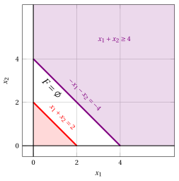
In red the half-plane \(x_1 + x_2 \le 2\) (with the non-negativity constraints) and in violet the half-plane \(x_1 + x_2 \ge 4\): their intersection is empty.

Example 5.5: unbounded LP problem

Consider the following LP problem in canonical maximization form with \(n=2\) non-negative variables and \(m=2\) less-than-or-equal-to linear constraints:

\[ \begin{array}{rrrrrrrrrrrrr} {\max} & \, {x_1} & {+} & \, {x_2} \\[1ex] \text{subject to} & {-} \, {x_1} & {+} & \, {x_2} & {\le} & {1} \\[1ex] & \, {x_1} & {-} & \, {x_2} & {\le} & {1} \\[1ex] & {x_1,} & & {x_2} & { \ge} & {0} \end{array} \]

For every value \(t \ge 0\), the point \(\bar{\boldsymbol x}(\, LP \,) = \begin{pmatrix} t \\[0.5ex] t \end{pmatrix}\) is a feasible solution, since

\[ - t + t = 0 \le 1, \qquad t - t = 0 \le 1, \qquad t \ge 0 \text{ and } t \ge 0 , \]

and its objective value is

\[ LB(\bar{\boldsymbol x}) = t + t = 2 \, t . \]

Accordingly, for every value \(M \in \R\), the feasible solution obtained with \(t > \frac{M}{2}\) has an objective value larger than \(M\), and then this LP problem is unbounded.

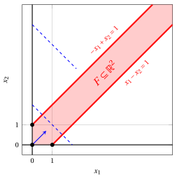
In dashed blue the level sets \(x_1 + x_2 = 2\) and \(x_1 + x_2 = 6\) of the objective function: the gradient points along the unbounded feasible region.

An LP problem whose feasible region \(F\) is unbounded is not necessarily an unbounded LP problem: the objective function may well attain a finite optimal value on \(F\).

Example 5.6: unbounded feasible region and multiple optimal solutions

Consider the following LP problem in canonical maximization form with \(n=2\) non-negative variables and \(m=2\) less-than-or-equal-to linear constraints:

\[ \begin{array}{rrrrrrrrrrrrr} {\max} & {-} \, {x_1} & {-} & \, {x_2} \\[1ex] \text{subject to} & {-} \, {x_1} & {-} & \, {x_2} & {\le} & {-2} \\[1ex] & \, {x_1} & {-} & \, {x_2} & {\le} & {2} \\[1ex] & {x_1,} & & {x_2} & { \ge} & {0} \end{array} \]

The feasible region \(F\) is unbounded. Nevertheless, the first constraint imposes \(x_1 + x_2 \ge 2\) for every feasible solution, and then

\[ - x_1 - x_2 \le -2, \qquad \forall \begin{pmatrix} x_1 \\ x_2\end{pmatrix} \in F . \]

The feasible solutions \(\begin{pmatrix} 0 \\ 2\end{pmatrix}\) and \(\begin{pmatrix} 2 \\ 0\end{pmatrix}\) attain this value, and then they are two optimal solutions and the optimal value is \(z(\, LP \,) = -2\).

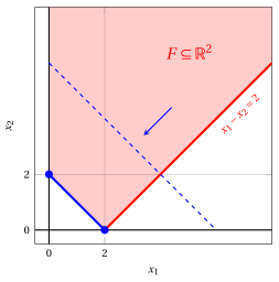
In dashed blue the level set \(-x_1 - x_2 = -6\) and in solid blue the level set \(-x_1 - x_2 = -2\), which contains the segment of optimal solutions joining the two blue vertices.

Observation 5.3: multiple optimal solutions

If \(\tilde{\boldsymbol x}^{(1)}(\, LP \,)\) and \(\tilde{\boldsymbol x}^{(2)}(\, LP \,)\) are two optimal solutions of an LP problem, then every point

\[ \lambda \, \tilde{\boldsymbol x}^{(1)}(\, LP \,) + (1-\lambda) \, \tilde{\boldsymbol x}^{(2)}(\, LP \,), \qquad \lambda \in [0,1], \]

is an optimal solution as well. Accordingly, an LP problem that admits an optimal solution admits either exactly one optimal solution or infinitely many optimal solutions.

Proof

Let \(\boldsymbol{x}^{\lambda} = \lambda \, \tilde{\boldsymbol x}^{(1)}(\, LP \,) + (1-\lambda) \, \tilde{\boldsymbol x}^{(2)}(\, LP \,)\) with \(\lambda \in [0,1]\). First, \(\boldsymbol{x}^{\lambda} \in F\). Indeed, the feasible region \(F\) is a polyhedron and, for each of its inequalities \({\boldsymbol a}\,{\boldsymbol x} \le b\), since \(\lambda \ge 0\), \(1-\lambda \ge 0\) and both solutions satisfy it, we have:

\[ {\boldsymbol a}\,\boldsymbol{x}^{\lambda} = \lambda \, {\boldsymbol a}\,\tilde{\boldsymbol x}^{(1)}(\, LP \,) + (1-\lambda) \, {\boldsymbol a}\,\tilde{\boldsymbol x}^{(2)}(\, LP \,) \le \lambda \, b + (1-\lambda) \, b = b ; \]

the same computation, with \(=\) in place of \(\le\), holds for each of its equalities. Moreover, since the objective function \(f\) is linear, we have:

\[\begin{align*} f(\boldsymbol{x}^{\lambda}) &= \lambda \, f(\tilde{\boldsymbol x}^{(1)}(\, LP \,)) + (1-\lambda) \, f(\tilde{\boldsymbol x}^{(2)}(\, LP \,)) \\[2ex] &= \lambda \, z(\, LP \,) + (1-\lambda) \, z(\, LP \,) = z(\, LP \,) , \end{align*}\]

where the second equality holds because both solutions are optimal. Accordingly, \(\boldsymbol{x}^{\lambda}\) is a feasible solution whose objective value is the optimal value, and then it is an optimal solution. □

5.3 Equivalent reformulations

• A generic LP problem may be written in a form which is neither the canonical maximization form (5.1) nor the standard maximization form (5.2): its objective function may have to be minimized, its constraints may be of the three types “\(\le\)”, “\(\ge\)” and “\(=\)”, and its variables may be non-positive or free.

• In this section we show that every generic LP problem can be rewritten in canonical maximization form and in standard maximization form.

Definition 5.4: equivalent LP problems

Two LP problems are called equivalent if, from an optimal solution of one of them, an optimal solution of the other one can be directly obtained, and the two problems are both infeasible, both unbounded, or both admit an optimal solution.

5.3.1 Minimization and maximization form

• For every linear function \(f\) and every polyhedron \(F\), we have:

  \[ \min \{\, f(\boldsymbol{x}) \;\text{subject to}\; \boldsymbol{x} \in F \,\} = - \max \{\, - f(\boldsymbol{x}) \;\text{subject to}\; \boldsymbol{x} \in F \,\} . \]

• Accordingly, an LP problem in minimization form with objective-function vector \({\boldsymbol c}\) is equivalent to the LP problem in maximization form with the same feasible region and objective-function vector \(-{\boldsymbol c}\):

  \[ \underbrace{\sum_{j=1}^n c_j \, x_j}_{{\boldsymbol c}' {\boldsymbol x}} \qquad \longrightarrow \qquad \underbrace{\sum_{j=1}^n (-c_j) \, x_j}_{-{\boldsymbol c}' {\boldsymbol x}} . \]

The two equivalent LP problems have the same optimal solutions, while their optimal values are opposite numbers:

\[ \tilde{\boldsymbol x}(\, LP_{\min} \,) = \tilde{\boldsymbol x}(\, LP_{\max} \,) \qquad \text{and} \qquad z(\, LP_{\min} \,) = - \, z(\, LP_{\max} \,) . \]

Example 5.7: from the minimization to the maximization form

Consider the following LP problem in minimization form with \(n=2\) non-negative variables:

\[ \begin{array}{rrrrrrrrrrrrr} {\min} & {2} \, {x_1} & {+} & {4} \, {x_2} \\[1ex] \text{subject to} & {-} \, {x_1} & {-} & \, {x_2} & {\le} & {-2} \\[1ex] & \, {x_1} & {-} & \, {x_2} & {\le} & {0} \\[1ex] & {x_1,} & & {x_2} & { \ge} & {0} \end{array} \]

By changing the sign of the objective-function vector, we obtain the equivalent LP problem in canonical maximization form of Example 5.2:

\[ \begin{array}{rrrrrrrrrrrrr} {\max} & {-2} \, {x_1} & {-} & {4} \, {x_2} \\[1ex] \text{subject to} & {-} \, {x_1} & {-} & \, {x_2} & {\le} & {-2} \\[1ex] & \, {x_1} & {-} & \, {x_2} & {\le} & {0} \\[1ex] & {x_1,} & & {x_2} & { \ge} & {0} \end{array} \]

The optimal solution of both problems is \(\tilde{\boldsymbol x}(\, LP \,) = \begin{pmatrix} 1 \\ 1 \end{pmatrix} ,\) while the optimal value of the minimization form is \(6\) and the optimal value of the maximization form is \(-6\).

5.3.2 Greater-than-or-equal-to and equality constraints

• A greater-than-or-equal-to linear constraint is equivalent to a less-than-or-equal-to linear constraint, since, by multiplying both sides by \(-1\), we have:

  \[ \sum_{j=1}^n a_{ij} \, x_j \ge b_i \qquad \Longleftrightarrow \qquad \sum_{j=1}^n (-a_{ij}) \, x_j \le - b_i . \]

• An equality linear constraint is equivalent to two less-than-or-equal-to linear constraints, since:

  \[ \sum_{j=1}^n a_{ij} \, x_j = b_i \qquad \Longleftrightarrow \qquad \underbrace{\sum_{j=1}^n a_{ij} \, x_j \le b_i}_{\text{first constraint}} \text{ and } \underbrace{\sum_{j=1}^n (-a_{ij}) \, x_j \le - b_i}_{\text{second constraint}} . \]

An LP problem (5.2) in standard maximization form with \(n\) non-negative variables and \(m\) equality linear constraints is equivalent to an LP problem (5.1) in canonical maximization form with the same \(n\) non-negative variables and \(2 \, m\) less-than-or-equal-to linear constraints:

\[\begin{align*} && \max \;\;{\sum_{j =1}^n c_j \, x_j} \\[1ex] && \text{subject to} \quad {\sum_{j =1}^n a_{ij} \, x_j} &\leq b_i, & \forall i \in \{1,2,\dots,m\}, \\[1ex] && {\sum_{j =1}^n (-a_{ij}) \, x_j} &\leq -b_i, & \forall i \in \{1,2,\dots,m\}, \\[1ex] &&x_j &\ge 0, & \forall j \in \{1,2,\dots,n\}. \end{align*}\]

The two LP problems have the same feasible region, and then the same optimal solutions and the same optimal value.

Example 5.8: from the standard to the canonical maximization form

Consider the LP problem in standard maximization form of Example 5.3, with \(n=3\) non-negative variables and \(m=1\) equality linear constraint:

\[ \begin{array}{rrrrrrrrrrrrr} {\max} & 2 \, {x_1} & {+} & 2 \, {x_2} & {+} & \, {x_3} \\[1ex] \text{subject to} & {2} \, {x_1} & {+} & 3 \, {x_2} & {+} & \, {x_3} & {=} & 4 \\[1ex] & {x_1,} & & {x_2,} & & {x_3} & { \ge} & {0} \end{array} \]

By replacing the equality linear constraint with two less-than-or-equal-to linear constraints, we obtain the equivalent LP problem in canonical maximization form with \(n=3\) non-negative variables and \(2 \, m = 2\) less-than-or-equal-to linear constraints:

\[ \begin{array}{rrrrrrrrrrrrr} {\max} & 2 \, {x_1} & {+} & 2 \, {x_2} & {+} & \, {x_3} \\[1ex] \text{subject to} & {2} \, {x_1} & {+} & 3 \, {x_2} & {+} & \, {x_3} & {\le} & 4 \\[1ex] & {-2} \, {x_1} & {-} & 3 \, {x_2} & {-} & \, {x_3} & {\le} & {-4} \\[1ex] & {x_1,} & & {x_2,} & & {x_3} & { \ge} & {0} \end{array} \]

5.3.3 Slack and surplus variables

• A less-than-or-equal-to linear constraint is equivalent to an equality linear constraint and a non-negativity constraint, obtained by adding one non-negative variable \(x_{n+i}\):

  \[ \sum_{j=1}^n a_{ij} \, x_j \le b_i \qquad \Longleftrightarrow \qquad \sum_{j=1}^n a_{ij} \, x_j + x_{n+i} = b_i \text{ and } x_{n+i} \ge 0 . \]

• A greater-than-or-equal-to linear constraint is equivalent to an equality linear constraint and a non-negativity constraint, obtained by subtracting one non-negative variable \(x_{n+i}\):

  \[ \sum_{j=1}^n a_{ij} \, x_j \ge b_i \qquad \Longleftrightarrow \qquad \sum_{j=1}^n a_{ij} \, x_j - x_{n+i} = b_i \text{ and } x_{n+i} \ge 0 . \]

Definition 5.5: slack and surplus variables

The additional non-negative variable \(x_{n+i}\) is called the slack variable of a less-than-or-equal-to linear constraint and the surplus variable of a greater-than-or-equal-to linear constraint. Its value measures, for a given feasible solution, the difference between the two sides of the constraint.

An LP problem (5.1) in canonical maximization form with \(n\) non-negative variables and \(m\) less-than-or-equal-to linear constraints is equivalent to an LP problem (5.2) in standard maximization form with \(n+m\) non-negative variables and the same \(m\) linear constraints, now equalities:

\[\begin{align*} && \max \;\;{\sum_{j =1}^n c_j \, x_j} \\[1ex] && \text{subject to} \quad {\sum_{j =1}^n a_{ij} \, x_j} + x_{n+i}&= b_i, & \forall i \in \{1,2,\dots,m\}, \\[1ex] &&x_j &\ge 0, & \forall j \in \{1,2,\dots,n+m\}. \end{align*}\]

• In matrix notation, the \(m\) slack variables form a column vector \({\boldsymbol x}_S \in \R^{m}_{\ge 0}\) and the constraint matrix of the standard maximization form is obtained by appending to \({\boldsymbol A}\) the identity matrix \({\boldsymbol I}\) of size \(m\):

  \[\begin{align*} && \max \;\;{\boldsymbol c}'\; {\boldsymbol x} \\[2ex] && \text{subject to} \quad \underbrace{{\boldsymbol A} \; {\boldsymbol x} +{\boldsymbol I} \; {\boldsymbol x}_S}_{ \begin{pmatrix} {\boldsymbol A} & {\boldsymbol I} \end{pmatrix} \begin{pmatrix} {\boldsymbol x} \\ {\boldsymbol x}_S \end{pmatrix} } &= {\boldsymbol b}, & \phantom{j=1111} \\[2ex] && {\boldsymbol x},~{\boldsymbol x}_S &\ge {\boldsymbol 0}, \end{align*}\]

  where

  \[ {\boldsymbol x}_S= \begin{pmatrix} x_{n+1} \\ x_{n+2} \\ \vdots \\ x_{n+m} \\ \end{pmatrix} \qquad\qquad {\boldsymbol I}= \begin{pmatrix} 1 & 0 & \dots & 0\\ 0 & 1 & \dots & 0\\ \vdots & \vdots & \ddots & \vdots \\ 0 & 0& \dots & 1 \end{pmatrix} \]

Example 5.9: from the canonical to the standard maximization form

By adding \(m=3\) slack variables, the LP problem of Example 5.1 becomes the following equivalent LP problem in standard maximization form with \(n+m=5\) non-negative variables:

\[ \begin{array}{rrrrrrrrrrrrrrr} {\max} & 5 \, {x_1} & {+} & 2 \, {x_2} \\[1ex] \text{subject to} & {-} \, {x_1} & {+} & 3 \, {x_2} & {+} & {x_3} & & & & & {=} & 12 \\[1ex] & {x_1} & {+} & 2 \, {x_2} & & & {+} & {x_4} & & & {=} & 12 \\[1ex] & 3 \, {x_1} & {-} & 2 \, {x_2} & & & & & {+} & {x_5} & {=} & 8 \\[1ex] & {x_1,} & & {x_2,} & & {x_3,} & & {x_4,} & & {x_5} & {\ge} & {0} \end{array} \]

The optimal solution \(\tilde{\boldsymbol x}(\, LP \,)\) of Example 5.1 satisfies the first constraint strictly and the other two with equality, and then the values of the three slack variables are \(\tilde{x}_3 = \frac{13}{2}\), \(\tilde{x}_4 = 0\) and \(\tilde{x}_5 = 0\).

5.3.4 Non-positive and free variables

• A non-positive variable \(x_j \le 0\) is equivalent to one non-negative variable \(x_j^{+} \ge 0\), by setting:

  \[ x_j = - \, x_j^{+} . \]

• A free variable \(x_j \gtreqless 0\) is equivalent to two non-negative variables \(x_j^{+} \ge 0\) and \(x_j^{-} \ge 0\), by setting:

  \[ x_j = x_j^{+} - x_j^{-} . \]

In both cases, the substitution is performed in the objective function and in every linear constraint of the LP problem. A free variable is replaced by two non-negative variables, since every real number is the difference of two non-negative numbers.

Example 5.10: equivalent LP problem with only non-negative variables

Consider the following LP problem with one non-negative variable \(x_1 \ge 0\), one non-positive variable \(x_2 \le 0\) and one free variable \(x_3 \gtreqless 0\):

\[ \begin{array}{rrrrrrrrrrrrr} {\max} & {2} \, {x_1} & {+} & {4} \, {x_2} & {+} & {2} \, {x_3} \\[2ex] \text{subject to} & {-} \, {x_1} & + & \, {x_2} & {+} & {x_3} & {=} & 2 \\[2ex] & {8} \, {x_1} & {+} & {2} \, {x_2} & & & {=} & {19} \\[2ex] & {x_1} & & & & & { \ge} & { 0 } \\[2ex] & & & {x_2} & & & { \le} & { 0 } \\[2ex] & & & & & {x_3} & { \gtreqless} & { 0 } \end{array} \]

By setting \(x_2 = -x_2^{+}\) and \(x_3 = x_3^{+} - x_3^{-}\), we obtain the following equivalent LP problem with only non-negative variables:

\[ \begin{array}{rrrrrrrrrrrrr} {\max} & {2} \, {x_1} & {-} & {4} \, {x_2^+} & {+} & {2} \, {x_3^+} & {-} & {2} \, {x_3^-} \\[2ex] \text{subject to} & {-} \, {x_1} & {-} & \, {x_2^+} & {+} & {x_3^+} & {-} & {x_3^-} & {=} & 2 \\[2ex] & {8} \, {x_1} & {-} & {2} \, {x_2^+} & & & & & {=} & {19} \\[2ex] & {x_1,} & & {x_2^+,} & & {x_3^+,} & & {x_3^-} & { \ge} & { 0 } \end{array} \]

From an optimal solution of the second LP problem, an optimal solution of the first one is obtained by computing \(\tilde{x}_2 = -\tilde{x}_2^{+}\) and \(\tilde{x}_3 = \tilde{x}_3^{+} - \tilde{x}_3^{-}\).

5.3.5 From a generic LP problem to the canonical and standard maximization form

Every generic LP problem can be rewritten in canonical maximization form and in standard maximization form by applying the following transformations:

	canonical max form	standard max form
\(\min {\boldsymbol c}' {\boldsymbol x}\)	\(-\max (-{\boldsymbol c})' {\boldsymbol x}\)	\(-\max (-{\boldsymbol c})' {\boldsymbol x}\)
\(\sum_j a_{ij} x_j \le b_i\)	unchanged	add a slack variable \(x_{n+i} \ge 0\)
\(\sum_j a_{ij} x_j \ge b_i\)	multiply by \(-1\)	subtract a surplus variable \(x_{n+i} \ge 0\)
\(\sum_j a_{ij} x_j = b_i\)	split into two “\(\le\)”, the second one multiplied by \(-1\)	unchanged
\(x_j \ge 0\)	unchanged	unchanged
\(x_j \le 0\)	\(x_j = -x_j^{+}\)	\(x_j = -x_j^{+}\)
\(x_j \gtreqless 0\)	\(x_j = x_j^{+} - x_j^{-}\)	\(x_j = x_j^{+} - x_j^{-}\)

Example 5.11: from a generic LP problem to the canonical maximization form

Consider the following generic LP problem with \(3\) variables:

\[ \begin{array}{rrrrrrrrrrrrr} {\min} & {3} \, {x_1} & {-} & {2} \, {x_2} & {+} & \, {x_3} \\[2ex] \text{subject to} & \, {x_1} & {+} & \, {x_2} & {-} & {x_3} & {\ge} & {4} \\[2ex] & {2} \, {x_1} & {-} & \, {x_2} & & & {=} & {6} \\[2ex] & {x_1} & & & & & { \ge} & { 0 } \\[2ex] & & & {x_2} & & & { \le} & { 0 } \\[2ex] & & & & & {x_3} & { \gtreqless} & { 0 } \end{array} \]

We apply the transformations of the table above:

1. the objective function is minimized, and then we maximize the opposite objective function;

2. the first constraint is a greater-than-or-equal-to constraint, and then we multiply it by \(-1\);

3. the second constraint is an equality constraint, and then we split it into two less-than-or-equal-to constraints;

4. the variable \(x_2\) is non-positive, and then we set \(x_2 = -x_2^{+}\) with \(x_2^{+} \ge 0\);

5. the variable \(x_3\) is free, and then we set \(x_3 = x_3^{+} - x_3^{-}\) with \(x_3^{+}, x_3^{-} \ge 0\).

We obtain the following equivalent LP problem in canonical maximization form with \(n=4\) non-negative variables and \(m=3\) less-than-or-equal-to linear constraints:

\[ \begin{array}{rrrrrrrrrrrrr} {-} {\max} & {-3} \, {x_1} & {-} & {2} \, {x_2^+} & {-} & \, {x_3^+} & {+} & \, {x_3^-} \\[2ex] \text{subject to} & {-} \, {x_1} & {+} & \, {x_2^+} & {+} & {x_3^+} & {-} & {x_3^-} & {\le} & {-4} \\[2ex] & {2} \, {x_1} & {+} & \, {x_2^+} & & & & & {\le} & {6} \\[2ex] & {-2} \, {x_1} & {-} & \, {x_2^+} & & & & & {\le} & {-6} \\[2ex] & {x_1,} & & {x_2^+,} & & {x_3^+,} & & {x_3^-} & { \ge} & { 0 } \end{array} \]

Finally, by adding \(m=3\) slack variables \(x_5, x_6, x_7\), we obtain the equivalent LP problem in standard maximization form with \(n+m=7\) non-negative variables and \(m=3\) equality linear constraints.

5.3.6 Rational input data

Definition 5.6: Least Common Denominator

Given a vector \({\boldsymbol v} \in \Q^{k}\) of \(k\) rational numbers \(v_j = \frac{p_j}{q_j}\) with \(p_j \in \Z\) and \(q_j \in \N\) coprime, \(\forall j \in \{1,2,\dots,k\}\), the Least Common Denominator ¹, denoted by \(lcd({\boldsymbol v})\), is the smallest positive integer number divisible by all the denominators \(q_j\), with \(j \in \{1,2,\dots,k\}\).

• Multiplying a linear constraint by a positive number does not change the set of points satisfying it, and multiplying the objective function by a positive number does not change the set of optimal solutions. Accordingly, an LP problem with rational input data is equivalent to an LP problem with integer input data.

Given an LP problem (5.1) with rational input data, the equivalent LP problem with integer input data reads as follows:

\[\begin{align*} && \frac{1}{lcd({\boldsymbol c})} \max \;\;{\sum_{j =1}^n lcd({\boldsymbol c}) \, c_j \, x_j} \\[2ex] && \text{subject to} \quad {\sum_{j =1}^n lcd([{\boldsymbol a}_i~b_i]) \, a_{ij} \, x_j} &\leq lcd([{\boldsymbol a}_i~b_i]) \, b_i, & \forall i \in \{1,2,\dots,m\}, \\[2ex] &&x_j &\ge 0, & \forall j \in \{1,2,\dots,n\}, \end{align*}\]

where \({\boldsymbol a}_i\) denotes the \(i\)-th row of the constraint matrix \({\boldsymbol A}\).

Example 5.12: equivalent LP problem with integer input data

For the following LP problem (5.1) with \(n=5\) non-negative variables, \(m=1\) less-than-or-equal-to linear constraint and rational input data:

\[ \begin{array}{rrrrrrrrrrrrr} {\max} & {\frac{1}{3}} \, {x_1} & {-} & {\frac{11}{27}} \, {x_2} & {+} & {\frac{7}{10}} \, {x_3} & {+} & {\frac{7}{5}} \, {x_4} & {+} & {\frac{2}{9}} \, {x_5} \\[2ex] \text{subject to} & {\frac{1}{2}} \, {x_1} & {+} & {\frac{3}{4}} \, {x_2} & {+} & {\frac{11}{6}} \, {x_3} & {-} & {\frac{1}{4}} \, {x_4} & {+} & {\frac{5}{2}} \, {x_5} & {\le} & {\frac{25}{12}} \\[2ex] & {x_1,} & & {x_2,} & & {x_3,} & & {x_4,} & & {x_5} & { \ge} & { 0 } \end{array} \]

we have:

\[ \underbrace{lcd\left(\begin{pmatrix} \frac{1}{3} \\[1ex] -\frac{11}{27} \\[1ex] \frac{7}{10} \\[1ex] \frac{7}{5} \\[1ex] \frac{2}{9} \end{pmatrix}\right)}_{=lcd({\boldsymbol c})} = 270 \text{ and } \underbrace{lcd\left(\begin{pmatrix} \frac{1}{2} \\[1ex] \frac{3}{4} \\[1ex] \frac{11}{6} \\[1ex] -\frac{1}{4} \\[1ex] \frac{5}{2} \\[1ex] \frac{25}{12} \end{pmatrix}\right)}_{= lcd \bigg( \left[ {\boldsymbol a}_1~\frac{25}{12} \right] \bigg)} = 12 \]

and, accordingly, the equivalent LP problem with the same variables and constraints and with integer input data reads as follows:

\[ \begin{array}{rrrrrrrrrrrrr} {\frac{1}{270}~~~} {\max} & {90} \, {x_1} & {-} & {110} \, {x_2} & {+} & {189} \, {x_3} & {+} & {378} \, {x_4} & {+} & {60} \, {x_5} \\[2ex] \text{subject to} & {6} \, {x_1} & {+} & {9} \, {x_2} & {+} & {22} \, {x_3} & {-} & {3} \, {x_4} & {+} & {30} \, {x_5} & {\le} & {25} \\[2ex] & {x_1,} & & {x_2,} & & {x_3,} & & {x_4,} & & {x_5} & { \ge} & { 0 } \end{array} \]

---

Exercises on this chapter: Possible outcomes and equivalent formulations

Interactive lab

The ideas of the chapter, hands on: move the sliders and drag the points. Each app also opens full page in the interactive lab: The outcomes of an LP problem.

---

1. or the Least Common Multiple of the denominators. ↩