Linear Programming problems¶

Part 1 · Linear functions, polyhedra and linear programming problems · Chapter 4 · Lecture notes, volume 1 (PDF) · Exercises: Linear Programming problems · App: The graphical method

4.1 Canonical maximization form¶

Definition 4.1: Linear Programming problems in canonical maximization form

Given:

an objective-function vector \({\boldsymbol c} \in \R^{n}\)
a constraint matrix \({\boldsymbol A} \in \R^{m \times n }\)
a right-hand-side (RHS) vector \({\boldsymbol b} \in \R^{m}\) with \(m\) rows

\[ \underbrace{ \begin{pmatrix} c_{1} \\ c_{2} \\ \vdots \\ \vdots \\ c_{n} \\ \end{pmatrix} }_{{\boldsymbol c}} \in \R^{n} \qquad \qquad \underbrace{ \begin{pmatrix} a_{11} & a_{12} & \dots & \dots & a_{1n}\\ a_{21} & a_{22} & \dots & \dots & a_{2n}\\ \vdots & \vdots & \ddots & \ddots & \vdots \\ a_{m1} & a_{m2} & \dots & \dots & a_{mn}\\ \end{pmatrix} }_{{\boldsymbol A}} \in \R^{m \times n } \qquad \qquad \underbrace{ \begin{pmatrix} b_{1} \\ b_{2} \\ \vdots \\ b_{m} \\ \end{pmatrix} }_{{\boldsymbol b}} \in \R^{m} \]

a Linear Programming problem LP in canonical maximization form with \(n\) non-negative variables

\[ \underbrace{ \begin{pmatrix} x_{1} \\ x_{2} \\ \vdots \\ \vdots \\ x_{n} \\ \end{pmatrix} }_{{\boldsymbol x}} \in \R^{n}_{\ge 0} \]

and \(m\) less-than-or-equal-to linear constraints is the following optimization problem:

\[\begin{align*} \label{ObjFunc} && \max \;\; \underbrace{\sum_{j =1}^n c_j \, x_j}_{ {\boldsymbol c}' {\boldsymbol x}} \qquad \qquad \qquad \qquad \qquad \qquad \tag{4.1a}\\[1ex] \label{Cons} && \text{subject to} \quad \underbrace{\sum_{j =1}^n a_{ij} \, x_j \le b_i, \qquad \forall i \in \{1,2,\dots,m\}}_{ {\boldsymbol A}\,{\boldsymbol x} \le {\boldsymbol b}}, \tag{4.1b}\\[1ex] \label{NonNegCons}&& \underbrace{x_j \ge 0, \qquad \forall j \in \{1,2,\dots,n\}}_{{\boldsymbol x} \ge {\boldsymbol 0}}, \tag{4.1c} \end{align*}\]

where \({\boldsymbol 0} = \begin{pmatrix} 0 \\ 0 \\ \vdots \\ 0 \\ \end{pmatrix}\) is a (column) vector of \(n\) zeros.

Example 4.1: LP problem in canonical maximization form

Consider the following input data of an LP problem with \(n=2\) and \(m=3\):

\[ {\boldsymbol c}= \begin{pmatrix} 5 \\[1ex] 2\\ \end{pmatrix} \qquad {\boldsymbol A}= \begin{pmatrix} -1 & 3 \\[1ex] 1 & 2 \\[1ex] 3 & -2 \\ \end{pmatrix} \qquad {\boldsymbol b}= \begin{pmatrix} 12 \\[1ex] 12 \\[1ex] 8\\ \end{pmatrix} \]

The numerical entries of the two column vectors and the matrix are

\[\begin{gather*} c_1=5,~c_2=2,~a_{11}=-1,~a_{12}=3,~a_{21}=1,~a_{22}=2,\\ a_{31}=3,~a_{32}=-2,~b_1=12,~b_2=12,~b_3=8. \end{gather*}\]

The problem involves \(n=2\) non-negative variables \({\boldsymbol x}= \begin{pmatrix} x_1 \\[1ex] x_2\\ \end{pmatrix}.\)

The associated LP problem in canonical maximization form with \(n=2\) non-negative variables and \(m=3\) less-than-or-equal-to linear constraints reads as follows:

\[ \begin{array}{rrrrrrrrrrrrr} {\max} & 5 \, {x_1} & {+} & 2 \, {x_2} \\[1ex] \text{subject to} & {-} \, {x_1} & {+} & 3 \, {x_2} & {\le} & 12 \\[1ex] & {x_1} & {+} & 2 \, {x_2} & {\le} & 12 \\[1ex] & {3} \, {x_1} & {-} & 2 \, {x_2} & {\le} & 8 \\[1ex] & {x_1,} & & {x_2} & { \ge} & {0} \end{array} \]

Example 4.2: LP problem in canonical maximization form

Consider the following input data of an LP problem with \(n=2\) and \(m=2\):

\[ {\boldsymbol c}= \begin{pmatrix} -2 \\[1ex] -4\\ \end{pmatrix} \qquad {\boldsymbol A}= \begin{pmatrix} -1 & -1 \\[1ex] 1 & -1 \\ \end{pmatrix} \qquad {\boldsymbol b}= \begin{pmatrix} -2 \\[1ex] 0\\ \end{pmatrix} \]

The numerical entries of the two column vectors and the matrix are

\[ c_1=-2,~c_2=-4,~a_{11}=-1,~a_{12}=-1,~a_{21}=1,~a_{22}=-1,~b_1=-2,~b_2=0. \]

The problem involves \(n=2\) non-negative decision variables \({\boldsymbol x}= \begin{pmatrix} x_1 \\[1ex] x_2\\ \end{pmatrix}.\)

The associated LP problem in canonical maximization form with \(n=2\) non-negative variables and \(m=2\) less-than-or-equal-to linear constraints reads as follows:

\[ \begin{array}{rrrrrrrrrrrrr} {\max} & {-2} \, {x_1} & {-} & 4\, {x_2} \\[1ex] \text{subject to} & {-} \, {x_1} & {-} & {x_2} & {\le} & {-2} \\[1ex] & {x_1} & {-} & {x_2} & {\le} & {0} \\[1ex] & {x_1,} & & {x_2} & { \ge} & {0} \end{array} \]

4.1.1 Feasible region and objective function¶

Definition 4.2: feasible region and objective function

The feasible region of an LP problem (4.1) is the polyhedron \(F\) defined as follows:

\[\begin{equation*} \label{FeasibleRegion} \begin{split} F = \left\{~ \underbrace{ \begin{pmatrix} x_{1} \\ x_{2} \\ \vdots \\ x_{n} \\ \end{pmatrix}}_{{\boldsymbol x}} \in \R^n : \right. ~~ & \underbrace{\sum_{j=1}^n a_{ij} \, x_j \le b_i,~~\forall i \in \{1,2,\dots,m\}}_{{\boldsymbol A}\,{\boldsymbol x} \le {\boldsymbol b}}, \\[1ex] & \left. \vphantom{\begin{pmatrix} x_{1} \\ x_{2} \\ \vdots \\ x_{n} \end{pmatrix}} \underbrace{x_j \ge 0,~~\forall j \in \{1,2,\dots,n\}}_{{\boldsymbol x} \ge {\boldsymbol 0}} ~\right\}. \end{split} \tag{4.2} \end{equation*}\]

The feasible region is defined by the less-than-or-equal-to linear constraints \(\eqref{Cons}\) and the non-negativity constraints \(\eqref{NonNegCons}\).
The objective function \(\eqref{ObjFunc}\) of an LP problem (4.1) to be maximized is the (scalar) linear function \(f\) defined as follows:

\[\begin{equation*} \label{ObjectiveFunction} f: \R^{n} \rightarrow \R, \qquad f : \underbrace{\begin{pmatrix} x_1 \\ x_2 \\ \vdots \\ x_n \end{pmatrix}}_{{\boldsymbol x}} \mapsto \underbrace{\sum_{j=1}^n c_j x_j}_{{\boldsymbol c}' {\boldsymbol x}} \tag{4.3} \end{equation*}\]

Example 4.3: objective function

The objective function of the LP problem of Example 4.1 is the scalar linear function:

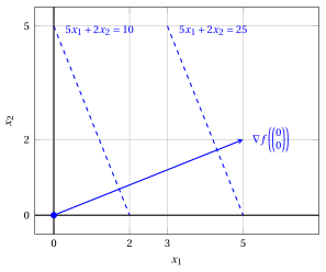
\[ f: \R^2 \rr \R, \quad f\!:\! \begin{pmatrix} x_1 \\[1ex] x_2 \end{pmatrix} \mapsto 5\,x_1 + 2\,x_2 \quad \text{its gradient is} \quad \nabla f\!\left( \begin{pmatrix} x_1\\[1ex] x_2 \end{pmatrix} \right) = \begin{pmatrix} 5 \\[1ex] 2 \end{pmatrix}. \]

Example 4.4: feasible region

The feasible region of the LP problem of Example 4.1 is the polyhedron:

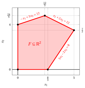
\[ F = \left\{~ \begin{pmatrix} x_1 \\[0.5ex] x_2 \end{pmatrix} \in \R^2 : -\,x_1 + 3x_2 \le 12,~~ x_1 + 2x_2 \le 12,~~ 3x_1 - 2x_2 \le 8,~~ x_1,\, x_2 \ge 0 ~\right\}. \]

4.1.2 Lower bounds¶

Definition 4.3: feasible solution and lower bound

Given

\[ \underbrace{\begin{pmatrix} \bar x_1 \\ \bar x_2 \\ \vdots \\ \bar x_n \end{pmatrix}}_{{ \bar{\boldsymbol x}}(\, LP \,)} \in F \]

a feasible solution of the LP problem (4.1) (a point satisfying constraints \(\eqref{Cons}\) and \(\eqref{NonNegCons}\)), we can compute a lower bound \(LB(\bar{\boldsymbol x})\) on the optimal value \(z(\, LP \,)\) as follows:

\[\begin{equation*} \label{FeasSolCanonical} LB(\bar{\boldsymbol x})= \sum_{j=1}^n c_j \; \bar{x}_j \tag{4.4} \end{equation*}\]

For every feasible solution \({ \bar{\boldsymbol x}}(\, LP \,) \in F\) of an LP problem (4.1), we have

\[\begin{equation*} LB(\bar{\boldsymbol x}) \le z(\, LP \,) \tag{4.5} \end{equation*}\]

Example 4.5: Feasible solutions and lower bounds

Consider the LP problem of Example 4.1. A feasible solution is for example \({ \bar{\boldsymbol x}}(\, LP \,)= \begin{pmatrix} 0 \\ 4 \end{pmatrix}\) (where \(\bar{x}_1=0\) and \(\bar{x}_2=4\)) since:

\[ - 0 + 3 \cdot 4 = 12 \le 12,~~~ 0 + 2 \cdot 4 = 8 \le 12,~~~ 3 \cdot 0 - 2 \cdot 4 = - 8 \le 8,~~~ 0\ge 0 \text{ and } 4 \ge 0 \]

Accordingly, a lower bound \(LB(\bar{\boldsymbol x})\) on the optimal value \(z(\, LP \,)\) of the LP problem is:

\[ LB(\bar{\boldsymbol x})= 5 \cdot 0 + 2 \cdot 4 = 8 \]

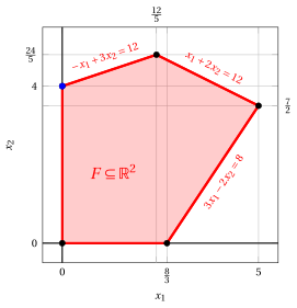
4.1.3 Graphical solution method¶

An optimal solution of an LP problem (4.1) in canonical maximization form with two variables can be graphically determined using the direction of the objective function gradient and the level sets perpendicular to the gradient.

Example 4.6: Graphical solution method

For the LP problem of Example 4.1:

\[ \begin{array}{rrrrrrrrrrrrr} {\max} & 5 \, {x_1} & {+} & 2 \, {x_2} \\[1ex] \text{subject to} & {-} \, {x_1} & {+} & 3 \, {x_2} & {\le} & 12 \\[1ex] & {x_1} & {+} & 2 \, {x_2} & {\le} & 12 \\[1ex] & {3} \, {x_1} & {-} & 2 \, {x_2} & {\le} & 8 \\[1ex] & {x_1,} & & {x_2} & { \ge} & {0} \end{array} \]

an optimal solution is:

\[ \underbrace{\begin{pmatrix} \tilde x_1\\[0.3ex] \tilde x_2 \end{pmatrix}}_{{ \tilde{\boldsymbol x}}(\, LP \,)} = \begin{pmatrix} 5\\[0.3ex] \frac{7}{2} \end{pmatrix} \]

and the optimal value is:

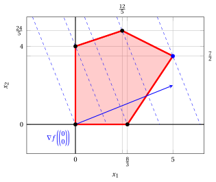
\[ z(\, LP \,)= 5\; \tilde{x}_1 + 2 \; \tilde{x}_2= 5 \cdot 5 + 2 \cdot \frac{7}{2} = 32 \]

In dashed blue, from left to right, the level sets \(5\,x_1 + 2\,x_2 = 0\), \(5\,x_1 + 2\,x_2 = 8\), \(5\,x_1 + 2\,x_2 = \frac{40}{3}\), \(5\,x_1 + 2\,x_2 = \frac{108}{5}\) and \(5\,x_1 + 2\,x_2 = 32\) of the objective function; the optimal vertex is depicted in blue.

Example 4.7: Graphical solution method

For the LP problem of Example 4.2:

\[ \begin{array}{rrrrrrrrrrrrr} {\max} & {-2} \, {x_1} & {-} & 4 \, {x_2} \\[1ex] \text{subject to} & {-} \, {x_1} & {-} & {x_2} & {\le} & {-2} \\[1ex] & {x_1} & {-} & {x_2} & {\le} & {0} \\[1ex] & {x_1,} & & {x_2} & { \ge} & {0} \end{array} \]

an optimal solution is:

\[ \underbrace{\begin{pmatrix} \tilde x_1\\[0.3ex] \tilde x_2 \end{pmatrix}}_{{ \tilde{\boldsymbol x}}(\, LP \,)} = \begin{pmatrix} 1\\[0.3ex] 1 \end{pmatrix} \]

and the optimal value is:

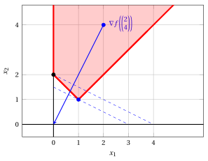
\[ z(\, LP \,) = -2\; \tilde{x}_1 - 4 \; \tilde{x}_2= -2 \cdot 1 - 4 \cdot 1 = -6 \]

In dashed blue, from bottom to top, the level sets \(-2\,x_1 - 4\,x_2 = -6\) and \(-2\,x_1 - 4\,x_2 = -8\) of the objective function; the optimal vertex \((1,1)\) is depicted in blue, and the gradient is drawn from the point \((2,4)\).

4.2 Standard maximization form¶

Definition 4.4: Linear Programming problems in standard maximization form

Given:

an objective-function vector \({\boldsymbol c} \in \R^{n}\)
a constraint matrix \({\boldsymbol A} \in \R^{m \times n }\)
a right-hand-side (RHS) vector \({\boldsymbol b} \in \R^{m}\) with \(m\) rows

\[ \underbrace{ \begin{pmatrix} c_{1} \\ c_{2} \\ \vdots \\ \vdots \\ c_{n} \\ \end{pmatrix} }_{{\boldsymbol c}} \in \R^{n} \qquad \qquad \underbrace{ \begin{pmatrix} a_{11} & a_{12} & \dots & \dots & a_{1n}\\ a_{21} & a_{22} & \dots & \dots & a_{2n}\\ \vdots & \vdots & \ddots & \ddots & \vdots \\ a_{m1} & a_{m2} & \dots & \dots & a_{mn}\\ \end{pmatrix} }_{{\boldsymbol A}} \in \R^{m \times n } \qquad \qquad \underbrace{ \begin{pmatrix} b_{1} \\ b_{2} \\ \vdots \\ b_{m} \\ \end{pmatrix} }_{{\boldsymbol b}} \in \R^{m} \]

a Linear Programming problem LP in standard maximization form with \(n\) non-negative variables

\[ \underbrace{ \begin{pmatrix} x_{1} \\ x_{2} \\ \vdots \\ \vdots \\ x_{n} \\ \end{pmatrix} }_{{\boldsymbol x}} \in \R^{n}_{\ge 0} \]

and \(m\) equality linear constraints is the following optimization problem:

\[\begin{align*} \label{STANDARD_ObjFunc} && \max \;\; \underbrace{\sum_{j =1}^n c_j \, x_j}_{ {\boldsymbol c}' {\boldsymbol x}} \qquad \qquad \qquad \qquad \qquad \qquad \tag{4.6a}\\[1ex] \label{STANDARD_Cons} && \text{subject to} \quad \underbrace{\sum_{j =1}^n a_{ij} \, x_j = b_i, \qquad \forall i \in \{1,2,\dots,m\}}_{ {\boldsymbol A}\,{\boldsymbol x} = {\boldsymbol b}}, \tag{4.6b}\\[1ex] \label{STANDARD_NonNegCons}&& \underbrace{x_j \ge 0, \qquad \forall j \in \{1,2,\dots,n\}}_{{\boldsymbol x} \ge {\boldsymbol 0}}, \tag{4.6c} \end{align*}\]

where \({\boldsymbol 0} = \begin{pmatrix} 0 \\ 0 \\ \vdots \\ 0 \\ \end{pmatrix}\) is a (column) vector of \(n\) zeros.

Example 4.8: LP problem in standard maximization form

Consider the following input data of an LP problem with \(n=3\) and \(m=1\):

\[ {\boldsymbol c}= \begin{pmatrix} 2 \\[1ex] 2\\[1ex] 1\\ \end{pmatrix} \qquad {\boldsymbol A}= \begin{pmatrix} 2 & 3 & 1 \end{pmatrix} \qquad {\boldsymbol b}= \begin{pmatrix} 4 \end{pmatrix} \]

The numerical entries of the two column vectors and the matrix are

\[ c_1=2,~c_2=2,~c_3=1,~a_{11}=2,~a_{12}=3,~a_{13}=1,~b_1=4. \]

The problem involves \(n=3\) non-negative variables \({\boldsymbol x}= \begin{pmatrix} x_1 \\[1ex] x_2 \\[1ex] x_3\\ \end{pmatrix}.\)

The associated LP problem in standard maximization form with \(n=3\) non-negative variables and \(m=1\) equality linear constraints reads as follows:

\[ \begin{array}{rrrrrrrrrrrrr} {\max} & 2 \, {x_1} & {+} & 2 \, {x_2} & {+} & \, {x_3} \\[1ex] \text{subject to} & {2} \, {x_1} & {+} & 3 \, {x_2} & {+} & \, {x_3} & {=} & 4 \\[1ex] & {x_1,} & & {x_2,} & & {x_3} & { \ge} & {0} \end{array} \]

4.2.1 Feasible region and objective function¶

Definition 4.5: feasible region and objective function

The feasible region of an LP problem (4.6) is the polyhedron \(F\) defined as follows:

\[\begin{equation*} \label{STANDARD_FeasibleRegion} \begin{split} F = \left\{~ \underbrace{ \begin{pmatrix} x_{1} \\ x_{2} \\ \vdots \\ x_{n} \\ \end{pmatrix}}_{{\boldsymbol x}} \in \R^n : \right. ~~ & \underbrace{\sum_{j=1}^n a_{ij} \, x_j = b_i,~~\forall i \in \{1,2,\dots,m\}}_{{\boldsymbol A}\,{\boldsymbol x} ={\boldsymbol b}}, \\[1ex] & \left. \vphantom{\begin{pmatrix} x_{1} \\ x_{2} \\ \vdots \\ x_{n} \end{pmatrix}} \underbrace{x_j \ge 0,~~\forall j \in \{1,2,\dots,n\}}_{{\boldsymbol x} \ge {\boldsymbol 0}} ~\right\}. \end{split} \tag{4.7} \end{equation*}\]

The feasible region is defined by the equality linear constraints \(\eqref{STANDARD_Cons}\) and the non-negativity constraints \(\eqref{STANDARD_NonNegCons}\).
The objective function \(\eqref{STANDARD_ObjFunc}\) of an LP problem (4.6) to be maximized is the (scalar) linear function \(f\) defined as follows:

\[\begin{equation*} \label{STANDARD_ObjectiveFunction} f: \R^{n} \rightarrow \R, \qquad f : \underbrace{\begin{pmatrix} x_1 \\ x_2 \\ \vdots \\ x_n \end{pmatrix}}_{{\boldsymbol x}} \mapsto \underbrace{\sum_{j=1}^n c_j x_j}_{{\boldsymbol c}' {\boldsymbol x}} \tag{4.8} \end{equation*}\]

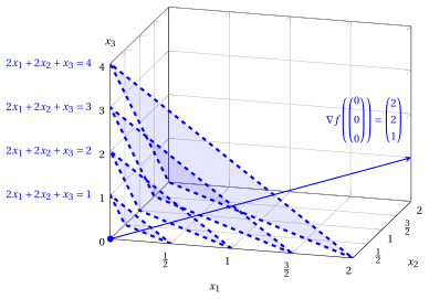
Example 4.9: objective function

The objective function of the LP problem of Example 4.8 is the scalar linear function:

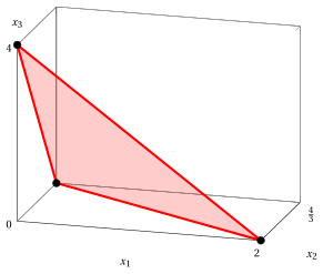
\[ f: \R^3 \rr \R, \quad f\!:\! \begin{pmatrix} x_1 \\[1ex] x_2 \\[1ex] x_3 \end{pmatrix} \mapsto 2\,x_1 + 2\,x_2 + x_3 \quad \text{and its gradient is} \quad \nabla f\!\left( \begin{pmatrix} x_1\\[1ex] x_2\\[1ex] x_3 \end{pmatrix} \right) = \begin{pmatrix} 2 \\[0.5ex] 2 \\[0.5ex] 1 \end{pmatrix}. \]

Example 4.10: feasible region

The feasible region of the LP problem of Example 4.8 is the polyhedron:

\[ F = \left\{~ \begin{pmatrix} x_1 \\[0.5ex] x_2 \\[0.5ex] x_3 \end{pmatrix} \in \R^3 : 2x_1 + 3x_2 + x_3 = 4,~~ x_1 \ge 0,~~ x_2 \ge 0,~~ x_3 \ge 0 ~\right\}. \]

4.2.2 Lower bounds¶

Definition 4.6: feasible solution and lower bound

Given

\[ \underbrace{\begin{pmatrix} \bar x_1 \\ \bar x_2 \\ \vdots \\ \bar x_n \end{pmatrix}}_{{ \bar{\boldsymbol x}}(\, LP \,)} \in F \]

a feasible solution of the LP problem (4.6) (a point satisfying constraints \(\eqref{STANDARD_Cons}\) and \(\eqref{STANDARD_NonNegCons}\)), we can compute a lower bound \(LB(\bar{\boldsymbol x})\) on the optimal value \(z(\, LP \,)\) as follows:

\[\begin{equation*} \label{FeasSolStandard} LB(\bar{\boldsymbol x})= \sum_{j=1}^n c_j \; \bar{x}_j \tag{4.9} \end{equation*}\]

For every feasible solution \({ \bar{\boldsymbol x}}(\, LP \,) \in F\) of an LP problem (4.6), we have

\[\begin{equation*} LB(\bar{\boldsymbol x}) \le z(\, LP \,) \tag{4.10} \end{equation*}\]

Example 4.11: Feasible solutions and lower bounds

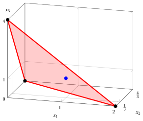
Consider the LP problem of Example 4.8. A feasible solution is for example \({ \bar{\boldsymbol x}}(\, LP \,)= \begin{pmatrix} 1 \\ \frac13 \\ 1 \end{pmatrix}\) (where \(\bar{x}_1 = 1\), \(\bar{x}_2 = \tfrac13\) and \(\bar{x}_3 = 1\)) since:

\[ 2\cdot 1 + 3\cdot \tfrac13 + 1 = 4, \qquad 1 \ge 0, \qquad \tfrac13 \ge 0, \qquad 1 \ge 0. \]

Accordingly, a lower bound \(LB(\bar{\boldsymbol x})\) on the optimal value \(z(\, LP \,)\) of the LP problem is:

\[ LB(\bar{\boldsymbol x}) = 2\cdot 1 + 2\cdot \tfrac13 + 1 = \frac{11}{3}. \]

4.2.3 Graphical solution method¶

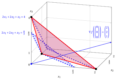
An optimal solution of an LP problem (4.6) in standard maximization form with two or three variables can be graphically determined using the direction of the objective function gradient and the level sets perpendicular to the gradient.

Example 4.12: Graphical solution method

For the LP problem of Example 4.8:

\[ \begin{array}{rrrrrrrrrrrrr} {\max} & 2 \, {x_1} & {+} & 2 \, {x_2} & {+} & \, {x_3} \\[1ex] \text{subject to} & {2} \, {x_1} & {+} & 3 \, {x_2} & {+} & \, {x_3} & {=} & 4 \\[1ex] & {x_1,} & & {x_2,} & & {x_3} & { \ge} & {0} \end{array} \]

All optimal solutions lie on the line segment

\[ \left\{\, \begin{pmatrix} x_1\\ x_2\\ x_3 \end{pmatrix} \in \R^3 \;:\; x_2 = 0,\; 2x_1 + x_3 = 4,\; x_1 \ge 0,\; x_3 \ge 0 \,\right\}, \]

i.e., on the segment joining the points \(\begin{pmatrix} 2\\ 0\\ 0 \end{pmatrix}\) and \(\begin{pmatrix} 0\\ 0\\ 4 \end{pmatrix}\). Taking for instance the optimal solution \(\tilde{\boldsymbol x}(\, LP \,) = \begin{pmatrix} 2\\ 0\\ 0 \end{pmatrix}\) (where \(\tilde{x}_1=2\), \(\tilde{x}_2=0\) and \(\tilde{x}_3=0\)), the optimal value is: \(z(\, LP \,) = 2\,\tilde{x}_1 + 2\,\tilde{x}_2 + \tilde{x}_3 = 2 \cdot 2 + 2 \cdot 0 + 0 = 4.\)

Exercises on this chapter: Linear Programming problems

Interactive lab¶

The ideas of the chapter, hands on: move the sliders and drag the points. Each app also opens full page in the interactive lab: The graphical method.