Simplex algorithm
Part 2 · The simplex algorithm · Chapter 6 · Lecture notes, volume 2 (PDF) · Exercises: Simplex algorithm · App: The simplex method step by step
6.1 The standard form of an LP problem in canonical max form
-
We consider an LP problem in standard maximization form with \(n+m\) non-negative variables and \(m\) equality linear constraints obtained from an LP problem in canonical maximization form with \(n\) non-negative variables and \(m\) less-than-or-equal-to linear constraints by adding \(m\) slack non-negative variables:
\[\begin{align*} && \max \;\;{\boldsymbol c}' \, {\boldsymbol x} \label{FORM_STANDARD_OBJ} \tag{6.1a}\\[2ex] && \text{subject to} \quad {\boldsymbol A} \; {\boldsymbol x} &= {\boldsymbol b}, & \phantom{j=1111} \label{FORM_STANDARD_CONS1} \tag{6.1b}\\[2ex] && {\boldsymbol x} &\ge {\boldsymbol 0}. \label{FORM_STANDARD_CONS2} \tag{6.1c} \end{align*}\]The input data of the LP problem are:
-
1. an objective-function column vector \({\boldsymbol c} \in \Z^{(n+m) }\) of \(n+m\) rows;
-
2. a constraint matrix \({\boldsymbol A} \in \Z^{m \times (n+m) }\) of \(m\) rows and \(n+m\) columns;
-
3. a right-hand side column vector \({\boldsymbol b} \in \Z^{m }\) of \(m\) rows.
\[ {\boldsymbol c}= \begin{pmatrix} c_{1} \\ c_{2} \\ \vdots \\ c_{n} \\ 0 \\ \vdots \\ 0 \\ \end{pmatrix} ~~~~~~ {\boldsymbol A}= \begin{pmatrix} a_{11} & a_{12} & \cdots & a_{1n} & 1 & 0 & \cdots & 0 \\ a_{21} & a_{22} & \cdots & a_{2n} & 0 & 1 & \cdots & 0 \\ \vdots & \vdots & \ddots & \vdots & \vdots & \vdots & \ddots & \vdots \\ a_{m1} & a_{m2} & \cdots & a_{mn} & 0 & 0 & \cdots & 1 \\ \end{pmatrix} ~~~~~~ {\boldsymbol b}= \begin{pmatrix} b_{1} \\ b_{2} \\ \vdots \\ b_{m} \\ \end{pmatrix} \]The \(m+n\) non negative variables can be written as a column vector \({\boldsymbol x}\) of \(n+m\) rows.
\[ {\boldsymbol x} = \begin{pmatrix} x_1 \\ x_2 \\ \vdots \\ x_n \\ x_{n+1} \\ x_{n+2} \\ \vdots \\ x_{n+m} \\ \end{pmatrix} \]Since the LP problem (6.1) is obtained by adding \(m\) slack variables to an LP problem in canonical form, we have:
\[ \begin{pmatrix} a_{1 (n+1)} & a_{1(n+2)} & \cdots &a_{1(n+m)}\\ a_{2(n+1)} & a_{2(n+2)} & \cdots &a_{2(n+m)}\\ \vdots & \vdots & \ddots & \vdots \\ a_{m(n+1)} & a_{m(n+2)} & \cdots &a_{m(n+m)}\\ \end{pmatrix} =\begin{pmatrix} 1 & 0 & \cdots & 0\\ 0 & 1 & \cdots & 0\\ \vdots & \vdots & \ddots & \vdots \\ 0 & 0& \cdots & 1 \end{pmatrix} \]which is the identity matrix \({\boldsymbol I}\) of size \(m\). Moreover, for the same reason, we have:
\[ \begin{pmatrix} c_{n+1} \\ c_{n+2} \\ \vdots \\ c_{n+m} \\ \end{pmatrix} = \begin{pmatrix} 0 \\ 0 \\ \vdots \\ 0 \\ \end{pmatrix} \] -
Since the constraint matrix \({\boldsymbol A} \in \Z^{m \times (n+m) }\) contains the identity matrix \({\boldsymbol I}\) of size \(m\), we have:
Accordingly there are \(m\) linearly independent rows and at least one set of \(m\) linearly independent columns 1 in the constraints matrix \({\boldsymbol A}\).
Example 6.1: standard max form of LP problems in canonical max form
We consider the following LP problem in canonical max form with \(n=2\) variables and \(m=3\) constraints:
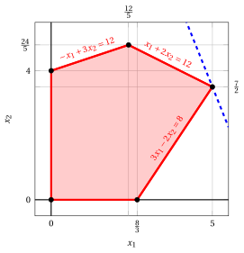
In dashed blue the level set \(5\,x_1 + 2\,x_2 = 32\) through the optimal vertex.
An optimal solution \({\tilde{\boldsymbol x}}(\,LP\,)\) is:
and the optimal value is:
The standard form with \(n+m=5\) variables and \(m=3\) constraints read as follows:
In the LP problem in standard form (called Example 6.1), we have:
An optimal solution \({\tilde{\boldsymbol x}}(\,LP\,)\) of the standard form is: \(\tilde{x}_1=5,~~\tilde{x}_2=\frac{7}{2},~~\tilde{x}_3=\frac{13}{2},~~\tilde{x}_4=0,~~\tilde{x}_5=0\).
6.2 Basis of the LP problem in standard form and dictionaries
Definition 6.1: basis of the LP problem
Given a subset \(\pazocal{B} \subseteq \{1,2,\dots,n+m\}\) of \(m\) indices of the \(n+m\) variables of the LP problem (6.1), if the matrix \({\boldsymbol A}_{\pazocal{B}} \in \R^{m \times m}\) containing the \(m\) columns of \({\boldsymbol A}\) with indices \(j \in \pazocal{B}\):
is invertible , it is called a basis of the LP problem (6.1).
Definition 6.2: partition of the indices, basic and non-basic variables
Given a basis \({\boldsymbol A}_{\pazocal{B}}\) of the LP problem (6.1), we have the following partition of the indices \(\{1,2,\dots,n+m\}\) of the variables:
Given a partition \(\pazocal{B}\) and \(\pazocal{N}\), we define:
-
the column vector of the basic variables containing the \(m\) variables with indices \(i \in \pazocal{B}\):
\[ {\boldsymbol x}_{\pazocal{B}}= (x_i)_{i \in \pazocal{B}} \] -
the column vector of the non-basic variables containing the \(n\) variables with indices \(i \in \pazocal{N}\):
\[ {\boldsymbol x}_{\pazocal{N}}=(x_i)_{i \in \pazocal{N}} \] -
the column vector \({\boldsymbol c}_{\pazocal{B}} \in \R^{m }\) containing the \(m\) values of \({\boldsymbol c}\) with indices \(i \in \pazocal{B}\):
\[ {\boldsymbol c}_{\pazocal{B}}=(c_i)_{i \in \pazocal{B}} \] -
the matrix \({\boldsymbol A}_{\pazocal{N}} \in \R^{m \times n}\) containing the \(n\) columns of \({\boldsymbol A}\) with indices \(j \in \pazocal{N}\):
\[ {\boldsymbol A}_{\pazocal{N}}=({\boldsymbol A}_j)_{j \in \pazocal{N}} \] -
the column vector \({\boldsymbol c}_{\pazocal{N}} \in \R^{n }\) containing the \(n\) values of \({\boldsymbol c}\) with indices \(i \in \pazocal{N}\):
\[ {\boldsymbol c}_{\pazocal{N}}=(c_i)_{i \in \pazocal{N}} \]
Example 6.2: Basis of LP problems, basic variables and non-basic variables
For the LP problem of Example 6.1 with \(\pazocal{B}= \{1,~~3,~~4\}\), we have:
and then \(\rank({\boldsymbol A}_{\pazocal{B}}) = 3\). Accordingly, the matrix \({\boldsymbol A}_{\pazocal{B}}\) is invertible and it is a basis of the LP problem. We compute the inverse matrix \({\boldsymbol A}_{\pazocal{B}}^{-1}\) with the method of Gauss-Jordan:
Since \(\pazocal{B}= \{1,~~3,~~4\}\), we have:
accordingly \(\pazocal{N}= \{2,~~5\}\) and we have:
Example 6.3: Basis of LP problems, basic variables and non-basic variables
For the LP problem of Example 6.1 with \(\pazocal{B}= \{1,~~2,~~4\}\), we have:
and
and then \(\rank({\boldsymbol A}_{\pazocal{B}}) = 3\). Accordingly, the matrix \({\boldsymbol A}_{\pazocal{B}}\) is invertible and it is a basis of the LP problem. We compute the inverse matrix \({\boldsymbol A}_{\pazocal{B}}^{-1}\) with the method of Gauss-Jordan:
Since \(\pazocal{B}= \{1,~~2,~~4\}\), we have:
accordingly \(\pazocal{N}= \{3,~~5\}\) and we have:
-
Given a basis \({\boldsymbol A}_{\pazocal{B}}\) of the LP problem (6.1), we can re-write the equality constraints \(\eqref{FORM_STANDARD_CONS1}\) as follows:
\[\begin{equation*} {\boldsymbol A} \; {\boldsymbol x} = \begin{pmatrix} {\boldsymbol A}_{\pazocal{B}} & {\boldsymbol A}_{\pazocal{N}} \end{pmatrix} \begin{pmatrix} {\boldsymbol x}_{\pazocal{B}} \\[1ex] {{\boldsymbol x}_{\pazocal{N}}} \end{pmatrix} ={\boldsymbol A}_{\pazocal{B}} \; {\boldsymbol x}_{\pazocal{B}} +{\boldsymbol A}_{\pazocal{N}} \; {{\boldsymbol x}_{\pazocal{N}}} = {\boldsymbol b} \end{equation*}\]and then, by multiplying by \({\boldsymbol A}_{\pazocal{B}}^{-1}\), we have:
\[\begin{align*} {\boldsymbol A}_{\pazocal{B}}^{-1} \big({\boldsymbol A}_{\pazocal{B}} \; {\boldsymbol x}_{\pazocal{B}} +{\boldsymbol A}_{\pazocal{N}} \; {{\boldsymbol x}_{\pazocal{N}}}\big) = {\boldsymbol A}_{\pazocal{B}}^{-1} \; {\boldsymbol b} &~~\Rightarrow~~ \underbrace{{\boldsymbol A}_{\pazocal{B}}^{-1}\;{\boldsymbol A}_{\pazocal{B}}}_{={\boldsymbol I}} \; {\boldsymbol x}_{\pazocal{B}} + {\boldsymbol A}_{\pazocal{B}}^{-1} \;{\boldsymbol A}_{\pazocal{N}} \; {{\boldsymbol x}_{\pazocal{N}}} = {\boldsymbol A}_{\pazocal{B}}^{-1} \; {\boldsymbol b} \end{align*}\]The basic variables can be written in function of the non-basic variables as follows:
\[\begin{equation*} {\boldsymbol x}_{\pazocal{B}} = {\boldsymbol A}_{\pazocal{B}}^{-1} \; {\boldsymbol b} - {\boldsymbol A}_{\pazocal{B}}^{-1}\;{\boldsymbol A}_{\pazocal{N}} \; {{\boldsymbol x}_{\pazocal{N}}} \label{BBBB} \tag{6.2} \end{equation*}\]Moreover, we can re-write the objective function \(\eqref{FORM_STANDARD_OBJ}\) value , denoted by \(z\), as follows:
\[\begin{equation*} z ={\boldsymbol c}' {\boldsymbol x}= \begin{pmatrix} {\boldsymbol c}_{\pazocal{B}} \\[1ex] {{\boldsymbol c}_{\pazocal{N}}} \end{pmatrix} ' \begin{pmatrix} {\boldsymbol x}_{\pazocal{B}} \\[1ex] {{\boldsymbol x}_{\pazocal{N}}} \end{pmatrix} = {\boldsymbol c}'_{\pazocal{B}} \; {\boldsymbol x}_{\pazocal{B}} + {\boldsymbol c}'_{\pazocal{N}} \;{{\boldsymbol x}_{\pazocal{N}}} \end{equation*}\]Using \(\eqref{BBBB}\), we then get:
\[ z = {\boldsymbol c}'_{\pazocal{B}} \; \big({\boldsymbol A}_{\pazocal{B}}^{-1} \; {\boldsymbol b} - {\boldsymbol A}_{\pazocal{B}}^{-1}\;{\boldsymbol A}_{\pazocal{N}} \; {{\boldsymbol x}_{\pazocal{N}}}\big) + {\boldsymbol c}'_{\pazocal{N}} \;{{\boldsymbol x}_{\pazocal{N}}} \]The objective function can be written in function of the non-basic variables as follows:
\[\begin{equation*} z = {\boldsymbol c}'_{\pazocal{B}} \; {\boldsymbol A}_{\pazocal{B}}^{-1}\;{\boldsymbol b} + \big({\boldsymbol c}'_{\pazocal{N}} - {\boldsymbol c}'_{\pazocal{B}} \; {\boldsymbol A}_{\pazocal{B}}^{-1}\;{\boldsymbol A}_{\pazocal{N}} \big) \; {{\boldsymbol x}_{\pazocal{N}}} \label{OOOO} \tag{6.3} \end{equation*}\]Using \(\eqref{BBBB}\) and \(\eqref{OOOO}\), the LP problem (6.1) can be reformulated in form of a dictionary.
Definition 6.3: dictionary
Given a basis \({\boldsymbol A}_{\pazocal{B}}\) of the LP problem (6.1), the associated dictionary is a system of \(m+1\) linear equations in which the basic variables and the objective function are written in function of the non-basic variables:
\[\begin{equation*} \begin{cases} {\boldsymbol x}_{\pazocal{B}} = {{\bar{\boldsymbol b}}} - {{\bar{\boldsymbol A}}} \; {{\boldsymbol x}_{\pazocal{N}}}\\[2ex] z = {\bar{z}} + { \bar{\boldsymbol c}}' \; {{\boldsymbol x}_{\pazocal{N}}} \end{cases} \qquad \text{where} \qquad \qquad \begin{cases} {{\bar{\boldsymbol b}}} = {\boldsymbol A}_{\pazocal{B}}^{-1} \; {\boldsymbol b}\\[2ex] {{\bar{\boldsymbol A}}} = {{\boldsymbol A}_{\pazocal{B}}^{-1} \;{\boldsymbol A}_{\pazocal{N}}}\\[2ex] {\bar{z}} = {\boldsymbol c}'_{\pazocal{B}} \; {\boldsymbol A}_{\pazocal{B}}^{-1} \; {\boldsymbol b} \\[2ex] {{ \bar{\boldsymbol c}}'} = {\boldsymbol c}'_{\pazocal{N}} - {\boldsymbol c}'_{\pazocal{B}} \; {\boldsymbol A}_{\pazocal{B}}^{-1} \;{\boldsymbol A}_{\pazocal{N}} \end{cases} \label{DICTIONARY} \tag{6.4} \end{equation*}\] -
Given a basis \({\boldsymbol A}_{\pazocal{B}}\) of the LP problem (6.1), in the associated dictionary there are:
-
the matrix \({\bar{\boldsymbol A}} \in \R^{m \times n}\) of \(m\) rows associated to the basic variables and \(n\) columns associated to the non-basic variables
-
two columns vectors \({\bar{\boldsymbol b}} \in \R^{m }\) and \({ \bar{\boldsymbol c}} \in \R^{n }\) of \(m\) rows associated to the basic variables and of \(n\) rows associated to the non-basic variables, respectively:
\[ {\bar{\boldsymbol A}} =(\bar{a}_{ij})_{i \in \pazocal{B}, j \in \pazocal{N}}, \qquad {\bar{\boldsymbol b}} =(\bar{b}_{i})_{i \in \pazocal{B}}, \qquad {\bar{\boldsymbol c}} =(\bar{c}_{i})_{i \in \pazocal{N}}. \]
A dictionary can be equivalently rewritten using the summations as follows:
\[\begin{equation*} \begin{cases} \displaystyle x_{i} = {{ \bar{b}_i}} - \sum_{j \in \pazocal{N}} \bar{a}_{ij} \; x_{j},~~ \forall i \in \pazocal{B}\\[4ex] \displaystyle z = \bar{z} + \sum_{j \in \pazocal{N}} \bar{c}_{j} \; x_{j} \end{cases} \end{equation*}\] -
Example 6.4: simplex dictionary
For the LP problem of Example 6.1, with \(\pazocal{B}= \{1,~~3,~~4\}\) and \(\pazocal{N}= \{2,~~5\},\) we have:
Accordingly, the associated dictionary is:
or, equivalently:
This dictionary is associated to the feasible solution \(\bar{x}_1=\frac{8}{3},\bar{x}_2=0,~\bar{x}_3=\frac{44}{3},~\bar{x}_4=\frac{28}{3},\bar{x}_5=0\) of value \(z=\frac{40}{3}\).
Example 6.5: simplex dictionary
For the LP problem of Example 6.1, with \(\pazocal{B}= \{1,~~2,~~4\}\) and \(\pazocal{N}= \{3,~~5\},\) we have:
Accordingly, the associated dictionary is:
or, equivalently:
This dictionary is not associated to a feasible solution.
6.2.1 Basic feasible solutions and reduced costs
-
The basic variable values depend on the non-basic variable values, accordingly:
-
the basic variables are the dependent variables
-
the non-basic variables are the independent variables
Definition 6.4: basic solution
Given a basis \({\boldsymbol A}_{\pazocal{B}}\) of the LP problem (6.1), by setting all the non-basic variables to zero we have:
\[\begin{equation*} {\boldsymbol x}_{\pazocal{B}} = {{\bar{\boldsymbol b}}} \text{ and } {\boldsymbol x}_{\pazocal{N}} = {\boldsymbol 0} \label{FEASIBLE_SOLUTIONS} \tag{6.5} \end{equation*}\]which is called a basic solution of the LP problem (6.1).
-
-
The variables are non-negative \(\eqref{FORM_STANDARD_CONS2}\) so not all basic solutions are feasible solutions.
Definition 6.5: basic feasible solutions
Given a basis \({\boldsymbol A}_{\pazocal{B}}\) of the LP problem (6.1), if \(~{{\bar{\boldsymbol b}}} \ge {\boldsymbol 0}~\) then
is called a basic feasible solution.
Definition 6.6: reduced cost vectors
Given a basis \({\boldsymbol A}_{\pazocal{B}}\) of the LP problem (6.1), the vector \({{ \bar{\boldsymbol c}}}\) is called the reduced costs vector.
-
The reduced cost
\[ \bar{c}_p=c_p - {\boldsymbol c}'_{\pazocal{B}} \; {\boldsymbol A}_{\pazocal{B}}^{-1} \;{\boldsymbol A}_{p} \]of a non-basic variable \(x_p\) with \(p \in \pazocal{N}\) is the change of the objective function per unit increment of the variable.
The increment is proportional to \(c_p\) while the decrement (due to the change of the basic variables to preserve the equality constraints \(\eqref{FORM_STANDARD_CONS1}\)) is proportional to \({\boldsymbol c}'_{\pazocal{B}} {\boldsymbol A}_{\pazocal{B}}^{-1} \;{\boldsymbol A}_{p}\).
6.2.2 Finding an initial basic feasible solution
For an LP problem (6.1), if \(~{\boldsymbol b} \ge {\boldsymbol 0}\), the partition:
is associated to a basis \({\boldsymbol A}_{\pazocal{B}}={\boldsymbol I}\) and to the initial basic feasible solution:
-
For an LP problem (6.1), since in \(\pazocal{B}\) there are the indices of the \(m\) slack variables, we have:
\[ {\boldsymbol A}_{\pazocal{B}}= \begin{pmatrix} 1 & 0 & \cdots & 0\\ 0 & 1 & \cdots & 0\\ \vdots & \vdots & \ddots & \vdots \\ 0 & 0& \cdots & 1 \end{pmatrix} ={\boldsymbol I} ={\boldsymbol A}_{\pazocal{B}}^{-1} \quad \text{ and } \quad {\boldsymbol c}_{\pazocal{B}} = \begin{pmatrix} 0 \\ 0 \\ \vdots \\ 0 \\ \end{pmatrix} \]Accordingly, the matrix \({\boldsymbol A}_{\pazocal{B}}\) is invertible and then it is a basis. Moreover, we have:
\[ {\boldsymbol A}_{\pazocal{N}}= \begin{pmatrix} a_{11} & a_{12} & \cdots & a_{1n}\\ a_{21} & a_{22} & \cdots & a_{2n}\\ \vdots & \vdots & \ddots & \vdots \\ a_{m1} & a_{m2} & \cdots & a_{mn}\\ \end{pmatrix} \quad \text{ and } \quad {\boldsymbol c}_{\pazocal{N}} = \begin{pmatrix} c_{1} \\ c_{2} \\ \vdots \\ c_{n} \\ \end{pmatrix} \]In these cases, we then have:
\[\begin{equation*} \begin{cases} {{\bar{\boldsymbol b}}} = {\boldsymbol A}_{\pazocal{B}}^{-1} \; {\boldsymbol b} = {\boldsymbol I} \; {\boldsymbol b} = {\boldsymbol b}\\[1ex] {{\bar{\boldsymbol A}}} = {{\boldsymbol A}_{\pazocal{B}}^{-1} \;{\boldsymbol A}_{\pazocal{N}}} = {\boldsymbol I} \; {\boldsymbol A}_{\pazocal{N}}= {\boldsymbol A}_{\pazocal{N}}\\[1ex] {\bar{z}} = {{\boldsymbol c}'_{\pazocal{B}} \; {\boldsymbol A}_{\pazocal{B}}^{-1}} \; {\boldsymbol b} = {{\boldsymbol c}'_{\pazocal{B}} \; {\boldsymbol I}} \; {\boldsymbol b} = 0\\[1ex] {{ \bar{\boldsymbol c}}'} = {{\boldsymbol c}'_{\pazocal{N}} - {{\boldsymbol c}'_{\pazocal{B}} \; {\boldsymbol A}_{\pazocal{B}}^{-1}} \;{\boldsymbol A}_{\pazocal{N}}} = {{\boldsymbol c}'_{\pazocal{N}} - {{\boldsymbol c}'_{\pazocal{B}} \; {\boldsymbol I}} \;{\boldsymbol A}_{\pazocal{N}}} = {\boldsymbol c}'_{\pazocal{N}} \end{cases} \end{equation*}\]
Example 6.6: initial basic feasible solution
For the LP problem of Example 6.1, since \(\begin{pmatrix} 12 \\ 12 \\ 8 \\ \end{pmatrix} \ge \begin{pmatrix} 0 \\ 0 \\ 0 \\ \end{pmatrix}\), with \(\pazocal{B}=\{3,4,5\}\) and \(\pazocal{N}=\{1,2\}\), we have the basic feasible solution \(\begin{pmatrix} x_3 \\ x_4 \\ x_5 \\ \end{pmatrix} = \begin{pmatrix} 12 \\ 12 \\ 8 \end{pmatrix}\) and \(\begin{pmatrix} x_1 \\ x_2 \end{pmatrix} = \begin{pmatrix} 0 \\ 0 \end{pmatrix}.\) Moreover \({\bar{z}}=0\) and we have:
and
6.3 Pivoting operations
- Given a basis \({\boldsymbol A}_{\pazocal{B}}\) and a basic feasible solution \({\boldsymbol x}_{\pazocal{B}} = {{\bar{\boldsymbol b}}}\) and \({\boldsymbol x}_{\pazocal{N}} = {\boldsymbol 0}\) of the LP problem (6.1), if in the associated dictionary there exists \(j \in \pazocal{N}\) such that \(\bar{c}_j > 0\) (a positive reduced cost), it is necessary to perform a pivoting operation.
Definition 6.7: pivoting operation
A pivoting operation consists in determining a new basic feasible solution with the goal of increasing the basic feasible solution value by swapping one non-basic variable and one basic variable.
-
The non-basic variable that becomes basic is called the pivot column
-
The basic variable that becomes non-basic is called the pivot row
6.3.1 Determining a new basic feasible solution
The pivot column is a non-basic variable with a positive reduced cost, i.e., a non-basic variable
-
Since only the value of the pivot column \(x_p\) with \(p \in \pazocal{N}\) is (potentially) increased among the non-basic variables, we have:
\[ {\boldsymbol x}_{\pazocal{B}} = {{\bar{\boldsymbol b}}} - \underbrace{{{\boldsymbol A}_{\pazocal{B}}^{-1} \;{\boldsymbol A}_{p}} }_{=\bar{\boldsymbol A}_{p}} \; x_{p} \]where \(\bar{\boldsymbol A}_{p}\) is the column of the matrix \({\bar{\boldsymbol A}}\) associated to the pivot column \(x_p\). These \(m\) equalities determine the change of the values of the basic variables caused by an increment of the value of the pivot column.
The value of the pivot column is increased as much as possible while at the same time maintaining non negative the value of all basic variables. In this way a new basic feasible solution is determined. Accordingly, the value of pivot column becomes the maximum value \(t\), called \(t_m\), such that:
\[ {{\bar{\boldsymbol b}}} - t \; \underbrace{{{\boldsymbol A}_{\pazocal{B}}^{-1} \;{\boldsymbol A}_{p}} }_{=\bar{\boldsymbol A}_{p} } \ge {\boldsymbol 0} \quad \Rightarrow \quad t_m=\min \left\{~\frac{\bar b_i}{\bar a_{ip}}: i\in\pazocal{B},~\bar a_{ip}>0 ~\right\} \]If \(\bar a_{ip}\le 0\) for every \(i\in\pazocal{B}\), then the LP problem is unbounded in the direction of \(x_p\). In this case, the value of the pivot column can be increased without bound while maintaining non negative the value of all basic variables.
Certificate of unboundedness. Given a basis \({\boldsymbol A}_{\pazocal{B}}\) with a basic feasible solution, if there exists a non-basic variable \(x_p\) with \(p \in \pazocal{N}\) such that
\[ \bar{c}_p > 0 \qquad \text{and} \qquad \bar{a}_{ip} \le 0, \quad \forall i \in \pazocal{B}, \]then the LP problem (6.1) is unbounded.
-
Indeed, for every value \(t \ge 0\), the point
\[\begin{equation*} \label{RAY} x_p = t, \qquad x_i = \bar{b}_i - t \; \bar{a}_{ip} ,\quad \forall i \in \pazocal{B}, \qquad x_j = 0 ,\quad \forall j \in \pazocal{N} \setminus \{p\}, \tag{6.8} \end{equation*}\]is a feasible solution of the LP problem (6.1): it satisfies the equality constraints \(\eqref{FORM_STANDARD_CONS1}\) by construction, and it satisfies the non-negativity constraints \(\eqref{FORM_STANDARD_CONS2}\) since \(\bar{b}_i \ge 0\) and \(- \, t \; \bar{a}_{ip} \ge 0\) for every \(i \in \pazocal{B}\).
-
The objective value of this feasible solution is
\[ \bar{z} + t \; \bar{c}_p , \]and then, for every value \(M \in \R\), the feasible solution obtained with \(t > \frac{M - \bar{z}}{\bar{c}_p}\) has an objective value larger than \(M\).
The pivot row is a basic variable whose value becomes zero by setting the value of the pivot column to \(t_m\), i.e., a basic variable
\[ x_r \text{ with } r \in \pazocal{B} \text{ such that } \bar{a}_{rp} > 0 \text{ and } \bar{b}_r - t_m \; \bar{a}_{rp} = 0 {\rm ~~(i.e.,~~} \frac{\bar{b}_r}{\bar{a}_{rp}} = t_m {\rm )} \]where \(\bar{a}_{rp}\) is the value of the column \(\bar{\boldsymbol A}_{p}\) associated to the basic variable \(x_r\).
-
-
Given \(t_m\) and \(\bar{\boldsymbol A}_{p}\), the new basic feasible solution (which determines the new vector \({\bar{\boldsymbol b}}\)) is obtained as follows:
\[\begin{equation*} \label{UPDATED2} x_i = \underbrace{\bar{b}_i - t_m \; \bar{a}_{ip}}_{\text{new } \bar{b}_i}, \quad \forall i \in \pazocal{B} \setminus \{r\}, \qquad x_p = \underbrace{t_m}_{\bar{b}_p}, \qquad x_r=0, \qquad x_j=0,\quad \forall j \in \pazocal{N}\setminus\{p\}. \tag{6.9} \end{equation*}\] -
Given a pivot column \(x_p\) with \(p \in \pazocal{N}\) and a pivot row \(x_r\) with \(r \in \pazocal{B}\), the new partition of the indices of the variables is updated as follows:
\[\begin{equation*} \label{UPDATED1} \pazocal{B} \leftarrow \big(\pazocal{B} \setminus \{ r \} \big) \cup \{ p \} \text{ and } \pazocal{N} \leftarrow \big(\pazocal{N} \setminus \{ p \} \big) \cup \{ r \} \tag{6.10} \end{equation*}\]By construction \({\boldsymbol A}_{\pazocal{B}}\) remains a basis.
Example 6.7: pivoting operations
For the LP problem of Example 6.1, with \(\pazocal{B}= \{3,~~4,~~5\}\) and \(\pazocal{N}= \{1,~~2\},\) we have:
Accordingly, we can choose \(x_1\) as the pivot column since \(\bar{c}_1 = 5 >0\). We then find the largest \(t\) such that \({{\bar{\boldsymbol b}}} - t \; \bar{\boldsymbol A}_1 \ge 0\):
The value of the pivot column becomes \(t_{m}\) and \(x_1=\frac{8}{3}\). The value of \(x_5\) becomes zero and \(x_5\) is the pivot row. The other basic variables take values \({ \bar{\boldsymbol b} } - t_{m} \; \bar{\boldsymbol A}_1\), then we have:
The new partition of the indices of the variables is \(\pazocal{B}=\{1,3,4\}\) and \(\pazocal{N}=\{2,5\}\).
In the same dictionary also \(\bar{c}_2 = 2 > 0\), so \(x_2\) can be chosen as the pivot column as well: the ratio test then gives \(t_m = 4\), the pivot row is \(x_3\) and the new partition is \(\pazocal{B}=\{2,4,5\}\) and \(\pazocal{N}=\{1,3\}\). The execution of the simplex algorithm that starts with this choice is worked out in the exercises of this chapter (Simplex algorithm with a different pivot column, problem \(P10\)).
Example 6.8: certificate of unboundedness
Consider the following LP problem in canonical maximization form with \(n=2\) non-negative variables and \(m=2\) less-than-or-equal-to linear constraints:
By adding \(m=2\) slack variables, with \(\pazocal{B}= \{3,~~4\}\) and \(\pazocal{N}= \{1,~~2\}\) we obtain the initial dictionary:
We perform one pivoting operation with pivot column \(x_1\) (since \(\bar{c}_1 = 1 > 0\)). The only positive value in the column of \(x_1\) is \(\bar{a}_{41} = 1\), and then \(t_m = \frac{1}{1} = 1\) and the pivot row is \(x_4\). With \(\pazocal{B}= \{1,~~3\}\) and \(\pazocal{N}= \{2,~~4\}\), the new dictionary is:
The reduced cost of the non-basic variable \(x_2\) is \(\bar{c}_2 = 2 > 0\), and the values of its column are
Accordingly, no pivot row can be determined and this LP problem is unbounded. The corresponding family of feasible solutions \(\eqref{RAY}\) is, for every value \(t \ge 0\):
whose objective value is \(1 + 2 \, t\).
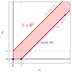
In violet the basic feasible solution reached after the first pivoting operation and the family of feasible solutions \(\eqref{RAY}\) along which the LP problem is unbounded.
6.3.2 Update of the dictionary
Once the pivot column \(x_p\) with \(p \in \pazocal{N}\) and the pivot row \(x_r\) with \(r \in \pazocal{B}\) are determined, the new dictionary can be determined by appropriate row operations to achieve the interchange.
-
Let \(x_p\) be the pivot column and \(x_r\) the pivot row. From the equation of the pivot row, we have:
\[ x_r=\bar b_r-\bar a_{rp}x_p-\sum_{j\in\pazocal{N}\setminus\{p\}}\bar a_{rj}x_j. \]Solving for \(x_p\) gives the equation of the pivot column in the new dictionary:
\[\begin{equation*} x_p=\frac{\bar b_r}{\bar a_{rp}} -\sum_{j\in\pazocal{N}\setminus\{p\}} \frac{\bar a_{rj}}{\bar a_{rp}}x_j -\frac{1}{\bar a_{rp}}x_r. \label{eq:pivot-equation} \tag{6.11} \end{equation*}\]For each remaining basic variable \(i\in\pazocal{B}\setminus\{r\}\), substituting with \(\eqref{eq:pivot-equation}\) gives their equations in the new dictionary:
\[\begin{equation*} x_i=\bar b_i -\sum_{j\in\pazocal{N}\setminus\{p\}}\bar a_{ij}x_j -\bar a_{ip} \left( \frac{\bar b_r}{\bar a_{rp}} -\sum_{j\in\pazocal{N}\setminus\{p\}} \frac{\bar a_{rj}}{\bar a_{rp}}x_j -\frac{1}{\bar a_{rp}}x_r \right). \label{eq:remaining-row-update} \tag{6.12} \end{equation*}\]For the objective function, substituting with \(\eqref{eq:pivot-equation}\) gives the equation of the objective function in the new dictionary:
\[\begin{equation*} z=\bar z +\sum_{j\in\pazocal{N}\setminus\{p\}}\bar c_jx_j +\bar c_p \left( \frac{\bar b_r}{\bar a_{rp}} -\sum_{j\in\pazocal{N}\setminus\{p\}} \frac{\bar a_{rj}}{\bar a_{rp}}x_j -\frac{1}{\bar a_{rp}}x_r \right). \label{eq:objective-update} \tag{6.13} \end{equation*}\]
Example 6.9: update of the dictionary
For the LP problem of Example 6.1, with \(\pazocal{B}= \{3,~~4,~~5\}\) and \(\pazocal{N}= \{1,~~2\},\) we have the dictionary:
Performing the pivot operation with \(x_1\) as the pivot column and \(x_5\) as the pivot row, we have:
Substituting in the other equations of the dictionary, we get:
Accordingly the new dictionary reads as follows:
This dictionary is associated to the feasible solution \(\bar{x}_1=\frac{8}{3},~\bar{x}_2=0,~\bar{x}_3=\frac{44}{3},~\bar{x}_4=\frac{28}{3},~\bar{x}_5=0\) of value \(z=\frac{40}{3}\).
6.4 High-level pseudo-code of the simplex algorithm
- The Phase \(0\) of the simplex algorithm consists in a procedure to determine an initial basic feasible solution and the associated initial dictionary. The Phase \(0\) is also able to prove that no basic feasible solution exists for an LP problem (6.1).
Algorithm
-
Input
An LP problem (6.1).
-
Output
An optimal solution of the LP problem (6.1), if one exists; otherwise, a certificate that the LP problem is infeasible or unbounded.
-
Step 0: Initialization
If \(b_i \ge 0\) for all \(i\in\{1,2,\ldots,m\}\), then set
\[ \pazocal B \leftarrow \{n+1,n+2,\ldots,n+m\}, \qquad \pazocal N \leftarrow \{1,2,\ldots,n\}, \]and consider the basic feasible solution
\[ x_i=\bar b_i,\quad \forall i\in\pazocal B, \qquad x_j=0,\quad \forall j\in\pazocal N, \]of the LP problem (6.1), together with the associated initial dictionary. Otherwise, execute Phase \(0\) of the simplex algorithm.
If Phase \(0\) proves that no basic feasible solution exists, then the LP problem is infeasible and
STOP. Otherwise, consider the basic feasible solution found by Phase \(0\) together with its dictionary. -
Step 1: Optimality check
With respect to the current dictionary
\[\begin{equation*} \begin{cases} \displaystyle x_i=\bar b_i-\sum_{j\in\pazocal N}\bar a_{ij}x_j, \qquad \forall i\in\pazocal B,\\[4ex] \displaystyle z=\bar z+\sum_{j\in\pazocal N}\bar c_jx_j, \end{cases} \end{equation*}\]check the reduced costs. If
\[ \bar c_j\le 0, \qquad \forall j\in\pazocal N, \]then the basic feasible solution
\[ x_i=\bar b_i,\quad \forall i\in\pazocal B, \qquad x_j=0,\quad \forall j\in\pazocal N, \]is an optimal solution and \(\bar z\) is the optimal value of the LP problem (6.1). In this case
STOP. -
Step 2: Pivoting operations
The pivot column is a non-basic variable \(x_p\) with \(p \in \pazocal{N}\) such that:
\[ \bar{c}_{p} > 0 \]-
a. If
\[ \bar a_{ip}\le 0, ~~~~ \forall i\in\pazocal{B}, \]then the LP problem (6.1) is unbounded.
STOP. -
b. Find the largest value \(t\) (called \(t_m\)) such that:
\[ \bar{b}_i - t \; \bar{a}_{ip} \ge 0, ~~~~ \forall i \in \pazocal{B} \quad \Rightarrow \quad t_m \leftarrow \min \left\{~\frac{\bar b_i}{\bar a_{ip}}: i\in\pazocal{B},~\bar a_{ip}>0 ~\right\} \]
The pivot row is a basic variable \(x_r\) with \(r \in \pazocal{B}\) such that:
\[ \bar{a}_{rp} > 0 \text{ and } \bar{b}_r - t_m \; \bar{a}_{rp} = 0 \]-
c. Update the dictionary with the new basis by performing the following operations:
-
The new equation of the pivot column \(x_p\) is obtained by isolating \(x_p\) in the pivot row:
\[\begin{equation*} x_p=\frac{\bar b_r}{\bar a_{rp}} -\sum_{j\in\pazocal{N}\setminus\{p\}} \frac{\bar a_{rj}}{\bar a_{rp}}x_j -\frac{1}{\bar a_{rp}}x_r. \end{equation*}\] -
The new equations of the basic variables \(x_i\) with \(i \in \pazocal{B}\setminus\{r\}\) are obtained by substituting the new equation of \(x_p\) in the old equations of \(x_i\):
\[\begin{equation*} x_i=\bar b_i -\sum_{j\in\pazocal{N}\setminus\{p\}}\bar a_{ij}x_j -\bar a_{ip} \left( \frac{\bar b_r}{\bar a_{rp}} -\sum_{j\in\pazocal{N}\setminus\{p\}} \frac{\bar a_{rj}}{\bar a_{rp}}x_j -\frac{1}{\bar a_{rp}}x_r \right). \end{equation*}\] -
The new equation of the objective function \(z\) is obtained by substituting the new equation of \(x_p\) in the old equation of \(z\):
\[\begin{equation*} z=\bar z +\sum_{j\in\pazocal{N}\setminus\{p\}}\bar c_jx_j +\bar c_p \left( \frac{\bar b_r}{\bar a_{rp}} -\sum_{j\in\pazocal{N}\setminus\{p\}} \frac{\bar a_{rj}}{\bar a_{rp}}x_j -\frac{1}{\bar a_{rp}}x_r \right). \end{equation*}\]
-
-
d. Update the basis with the new partition of the indices of the variables:
\[ \pazocal{B} \leftarrow \big(\pazocal{B} \setminus \{ r \} \big) \cup \{ p \} \text{ and } \pazocal{N} \leftarrow \big(\pazocal{N} \setminus \{ p \} \big) \cup \{ r \} \]
go to step \(1\).
-
Example 6.10: execution of the simplex algorithm
We execute the simplex algorithm on the LP problem of Example 6.1. Since \({\boldsymbol b} \ge {\boldsymbol 0}\), the initial basic feasible solution is the one of Example 6.6, associated with \(\pazocal{B}=\{3,4,5\}\) and \(\pazocal{N}=\{1,2\}\).
-
Initialization
Consider the initial dictionary:
\[\begin{equation*} \begin{cases} \begin{array}{rrrrrrrrrrrrr} {x_3} & {=} & {12} & {+} & {x_1} & {-} & {3\,x_2} \\[2ex] {x_4} & {=} & {12} & {-} & {x_1} & {-} & {2\;x_2} \\[2ex] {x_5} & {=} & {8} & {-} & {3\,x_1} & {+} & {2\;x_2} \\[2ex] {z} & {=} & {0} & {+} & {5\,x_1} & {+} & {2\,x_2} \end{array} \end{cases} \end{equation*}\]where \(\pazocal{B}=\{3,4,5\}\) and \(\pazocal{N}=\{1,2\}\). The basic feasible solution is:
\[ \bar x_3=12,~~ \bar x_4=12,~~ \bar x_5=8,~~~~~ \bar x_1=0,~~ \bar x_2=0~~ ~~~\text{of value } 0 \] -
Iteration 1
If we increase the value of the variable \(x_1\), we can get a better solution. We have:
\[ \begin{cases} x_3 &= 12 + x_1 \\[2ex] x_4 &= 12 - x_1 \\[2ex] x_5 &= 8 - 3\: x_1 \end{cases} \qquad \qquad \begin{cases} \underbrace{ 12 + x_1 \ge 0}_{x_3 \ge 0} \\[2ex] \underbrace{ 12 - x_1 \ge 0}_{x_4 \ge 0} \\[2ex] \underbrace{ 8 - 3\: x_1 \ge 0}_{x_5 \ge 0} \end{cases} \qquad \qquad \begin{cases} x_1 &\ge -12 \\[2ex] x_1 &\le 12 \\[2ex] x_1 &\le \dfrac{8}{3} \end{cases} \]By increasing the value of \(x_1\) to \(\min \left\{12,\dfrac{8}{3}\right\}=\dfrac{8}{3}\), the value of \(x_5\) decreases to 0.
Then, we have that:
- \(x_1\) becomes basic and accordingly \(x_5\) becomes non-basic
We have:
\[ x_5 = 8 - 3\; x_1 + 2\; x_2 \text{ then } x_1= \dfrac{8}{3} +\dfrac{2}{3}\: x_2 -\dfrac{1}{3}\: x_5. \]Substituting in the other equations of the dictionary, we get:
\[ x_3 = 12 + \left(\dfrac{8}{3} +\dfrac{2}{3}\: x_2 -\dfrac{1}{3}\: x_5 \right) - 3 \:x_2= \dfrac{44}{3} -\dfrac{7}{3}\: x_2 -\dfrac{1}{3}\: x_5 \]\[ x_4 = 12 - \left(\dfrac{8}{3} +\dfrac{2}{3}\: x_2 -\dfrac{1}{3}\: x_5 \right) - 2 \:x_2= \dfrac{28}{3} -\dfrac{8}{3}\: x_2 +\dfrac{1}{3}\: x_5 \]\[ z = 5 \: \left(\dfrac{8}{3} +\dfrac{2}{3}\: x_2 -\dfrac{1}{3}\: x_5 \right) + 2 \: x_2 = \dfrac{40}{3} +\dfrac{16}{3}\: x_2 -\dfrac{5}{3}\: x_5 \] -
Iteration 2
Consider the dictionary:
\[\begin{equation*} \begin{cases} \begin{array}{rrrrrrrrrrrrr} {x_1} & {=} & {\dfrac{8}{3}} & {+} & {\dfrac{2}{3}}\, {x_2} & {-} & {\dfrac{1}{3}}\, {x_5} \\[2ex] {x_3} & {=} & {\dfrac{44}{3}} & {-} & {\dfrac{7}{3}}\, {x_2} & {-} & {\dfrac{1}{3}}\, {x_5} \\[2ex] {x_4} & {=} & {\dfrac{28}{3}} & {-} & {\dfrac{8}{3}}\, {x_2} & {+} & {\dfrac{1}{3}}\, {x_5} \\[2ex] {z} & {=} & {\dfrac{40}{3}} & {+} & {\dfrac{16}{3}}\, {x_2} & {-} & {\dfrac{5}{3}}\, \, {x_5} \end{array} \end{cases} \end{equation*}\]where \(\pazocal{B}=\{1,3,4\}\) and \(\pazocal{N}=\{2,5\}\). The basic feasible solution is:
\[ \bar x_1=\dfrac{8}{3},~~ \bar x_3=\dfrac{44}{3},~~ \bar x_4=\dfrac{28}{3},~~~~ \bar x_2=0,~~ \bar x_5=0 ~~~\text{of value } \dfrac{40}{3} \]If we increase the value of the variable \(x_2\), we can get a better solution. We have:
\[ \begin{cases} x_1 &= \dfrac{8}{3} + \dfrac{2}{3}\: x_2 \\[2ex] x_3 &= \dfrac{44}{3} - \dfrac{7}{3}\: x_2\\[2ex] x_4 &= \dfrac{28}{3} - \dfrac{8}{3}\: x_2 \end{cases} \qquad \qquad \begin{cases} \overbrace{ \dfrac{8}{3} + \dfrac{2}{3}\: x_2 \ge 0}^{x_1 \ge 0} \\[2ex] \underbrace{ \dfrac{44}{3} - \dfrac{7}{3}\: x_2 \ge 0}_{x_3 \ge 0}\\[2ex] \underbrace{ \dfrac{28}{3} - \dfrac{8}{3}\: x_2 \ge 0}_{x_4 \ge 0} \end{cases} \qquad \qquad \begin{cases} x_2 &\ge -4 \\[2ex] x_2 &\le \dfrac{44}{7} \\[2ex] x_2 &\le \dfrac{7}{2} \end{cases} \]By increasing the value of \(x_2\) to \(\min \left\{\dfrac{44}{7},\dfrac{7}{2}\right\}=\dfrac{7}{2}\), the value of \(x_4\) decreases to 0.
Then, we have that:
- \(x_2\) becomes basic and accordingly \(x_4\) becomes non-basic
We have:
\[ x_4 = \dfrac{28}{3} -\dfrac{8}{3}\: x_2 +\dfrac{1}{3}\: x_5 \text{ then } x_2= \dfrac{7}{2} -\dfrac{3}{8}\: x_4 +\dfrac{1}{8}\: x_5. \]Substituting in the other equations of the dictionary, we get:
\[ x_1 = \dfrac{8}{3} + \dfrac{2}{3} \; \left( \dfrac{7}{2} -\dfrac{3}{8}\: x_4 +\dfrac{1}{8}\: x_5 \right) - \dfrac{1}{3} \:x_5= 5 -\dfrac{1}{4}\: x_4 - \dfrac{1}{4}\: x_5 \]\[ x_3 = \dfrac{44}{3} - \dfrac{7}{3} \; \left( \dfrac{7}{2} -\dfrac{3}{8}\: x_4 +\dfrac{1}{8}\: x_5 \right) - \dfrac{1}{3} \:x_5= \dfrac{13}{2} +\dfrac{7}{8}\: x_4 - \dfrac{5}{8}\: x_5 \]\[ z = \dfrac{40}{3} + \dfrac{16}{3} \; \left( \dfrac{7}{2} -\dfrac{3}{8}\: x_4 +\dfrac{1}{8}\: x_5 \right) -\dfrac{5}{3}\: x_5 = 32 -2\: x_4 -x_5 \]Accordingly, we obtained an optimal solution and this is the optimal dictionary:
\[\begin{equation*} \begin{cases} \begin{array}{rrrrrrrrrrrrr} {x_1=5} & {-} & {\dfrac{1}{4}} \, {x_4} & {-} & {\dfrac{1}{4}}\, {x_5} \\[2ex] {x_2=\dfrac{7}{2}} & {-} & {\dfrac{3}{8}}\, {x_4} & {+} & {\dfrac{1}{8}}\, {x_5} \\[2ex] {x_3=\dfrac{13}{2}} & {+} & {\dfrac{7}{8}}\, {x_4} & {-} & {\dfrac{5}{8}}\, {x_5} \\[2ex] {z= 32} & {-} & {2} \, {x_4} & {-} & \, {x_5} \end{array} \end{cases} \end{equation*}\]where \(\pazocal{B}=\{1,2,3\}\) and \(\pazocal{N}=\{4,5\}\). The optimal solution is:
\[ \tilde{x}_1=5,~~ \tilde{x}_2=\dfrac{7}{2},~~ \tilde{x}_3=\dfrac{13}{2},~~~~~ \tilde{x}_4=0,~~ \tilde{x}_5=0 ~~~\text{of value } 32 \]
The feasible region of the LP problem (in canonical form) is the polyhedron shaded in red:
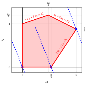
In violet the first and the second vertex explored by this execution of the simplex algorithm (before reaching the optimal one depicted in blue).
In dashed blue, the contour lines \(5\,x_1 + 2\,x_2 = 0\), \(5\,x_1 + 2\,x_2 = \frac{40}{3}\) and \(5\,x_1 + 2\,x_2 = 32\) of the objective function associated to the values taken in the three vertices.
At the first iteration the pivot column \(x_1\) was chosen among the two non-basic variables with a positive reduced cost. Choosing \(x_2\) instead, the simplex algorithm reaches the same optimal solution after three pivoting operations, visiting the vertices \((0,4)\) and \(\left(\frac{12}{5},\frac{24}{5}\right)\): the choice of the pivot column changes the path on the polyhedron and the number of iterations (see the exercise Simplex algorithm with a different pivot column, problem \(P10\)).
Exercises on this chapter: Simplex algorithm
Interactive lab
The ideas of the chapter, hands on: move the sliders and drag the points. Each app also opens full page in the interactive lab: The simplex method step by step.
-
The row rank and the column rank of a matrix are equal ↩