Linear functions

Part 1 · Linear functions, polyhedra and linear programming problems · Chapter 1 · Lecture notes, volume 1 (PDF) · App: Level lines

1.1 Linear functions

Definition 1.1: linear function

Given a (column) vector

\[ \underbrace{ \begin{pmatrix} c_1 \\ c_2 \\ \vdots \\ c_n \end{pmatrix}}_{ {\boldsymbol c}} \in \mathbb{R}^{n} \]

the associated (scalar) function

\[\begin{align*} f: \mathbb{R}^{n} \rightarrow \mathbb{R}, ~~~ f:\underbrace{\begin{pmatrix} x_1 \\ x_2 \\ \vdots \\ x_n \end{pmatrix}}_{{\boldsymbol x}} \mapsto \underbrace{\sum_{j=1}^n c_j x_j}_{{\boldsymbol c}' {\boldsymbol x}} \tag{1.1} \end{align*}\]

is called a linear function.

Definition 1.2: gradient of a linear function

The gradient (vector of the partial derivatives) of the linear function \(f({\boldsymbol x}) = {\boldsymbol c}'{\boldsymbol x}\) is:

\[\begin{align*} \nabla f({\boldsymbol x}) &= \begin{pmatrix} \frac{ \partial f({\boldsymbol x})}{ \partial x_1} \\[1ex] \frac{ \partial f({\boldsymbol x})}{ \partial x_2} \\[1ex] \vdots \\[1ex] \frac{ \partial f({\boldsymbol x})}{ \partial x_n} \end{pmatrix} = \underbrace{\begin{pmatrix} c_1 \\[1ex] c_2 \\[1ex] \vdots \\[1ex] c_n \end{pmatrix}}_{ {\boldsymbol c}} \end{align*}\]

Definition 1.3: Hessian of a linear function

The Hessian (matrix of the second partial derivatives) of the linear function \(f({\boldsymbol x}) = {\boldsymbol c}'{\boldsymbol x}\) is the \(n \times n\) matrix:

\[\begin{align*} \nabla^2 f({\boldsymbol x}) = \begin{pmatrix} \frac{\partial^2 f({\boldsymbol x})}{\partial x_1 \partial x_1} & \frac{\partial^2 f({\boldsymbol x})}{\partial x_1 \partial x_2} & \cdots & \frac{\partial^2 f({\boldsymbol x})}{\partial x_1 \partial x_n} \\[1.5ex] \frac{\partial^2 f({\boldsymbol x})}{\partial x_2 \partial x_1} & \frac{\partial^2 f({\boldsymbol x})}{\partial x_2 \partial x_2} & \cdots & \frac{\partial^2 f({\boldsymbol x})}{\partial x_2 \partial x_n} \\[1.5ex] \vdots & \vdots & \ddots & \vdots \\[1.5ex] \frac{\partial^2 f({\boldsymbol x})}{\partial x_n \partial x_1} & \frac{\partial^2 f({\boldsymbol x})}{\partial x_n \partial x_2} & \cdots & \frac{\partial^2 f({\boldsymbol x})}{\partial x_n \partial x_n} \end{pmatrix} = \begin{pmatrix} 0 & 0 & \cdots & 0 \\[1ex] 0 & 0 & \cdots & 0 \\[1ex] \vdots & \vdots & \ddots & \vdots \\[1ex] 0 & 0 & \cdots & 0 \end{pmatrix} \end{align*}\]

since every first partial derivative \(\frac{\partial f({\boldsymbol x})}{\partial x_j} = c_j\) is a constant.

Definition 1.4: level sets of a linear function

The level sets of the linear function \(f({\boldsymbol x}) = {\boldsymbol c}'{\boldsymbol x}\) (the sets of points in which the function is constant) are:

\[\begin{align*} \left\{~~{\boldsymbol x} \in \R^{n}:~~ {\boldsymbol c}' \; {\boldsymbol x}= k ~~\right\} , \qquad \forall k \in \mathbb{R} \end{align*}\]

• The gradient of a linear function is the same vector \({\boldsymbol c}\) at every point and, accordingly, its Hessian (matrix of the second partial derivatives) is the zero matrix everywhere.

• The level sets of a linear function are the hyperplanes perpendicular to the gradient.

Example 1.1: gradient and level sets of linear functions

With \({\boldsymbol c}=\begin{pmatrix} 8\\ 4 \end{pmatrix}\), the associated linear function is:

\[ f: \mathbb{R}^{2} \rightarrow \mathbb{R},~~ f: \begin{pmatrix} x_1 \\ x_2 \\ \end{pmatrix} \mapsto \begin{pmatrix} 8 & 4 \\ \end{pmatrix} \; \begin{pmatrix} x_{1} \\ x_{2} \\ \end{pmatrix}= 8\:x_1 + 4\: \, x_2 \]

Gradient:

\[ \nabla f\left(\begin{pmatrix} x_1 \\ x_2 \\ \end{pmatrix}\right) = \begin{pmatrix} 8 \\[0.5ex] 4 \end{pmatrix} \]

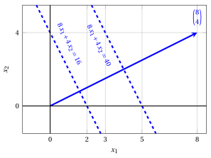
The figure shows:

• The gradient evaluated at \(\begin{pmatrix} 0 \\ 0 \end{pmatrix}\): \(\nabla f\left(\begin{pmatrix} 0 \\ 0 \end{pmatrix}\right) =\begin{pmatrix} 8 \\[0.5ex] 4 \end{pmatrix}\) (blue arrow)

• Two level sets (blue dashed lines): \(8 x_1 +4 x_2 = 16\) and \(8 x_1 +4 x_2 = 40\)

Example 1.2: gradient and level sets of linear functions

With \({\boldsymbol c}=\begin{pmatrix} -8\\ -4 \end{pmatrix}\), the associated linear function is:

\[ f: \mathbb{R}^{2} \rightarrow \mathbb{R},~~ f: \begin{pmatrix} x_1 \\ x_2 \\ \end{pmatrix} \mapsto \begin{pmatrix} -8 & -4 \\ \end{pmatrix} \; \begin{pmatrix} x_{1} \\ x_{2} \\ \end{pmatrix}= -8\:x_1 - 4\: \, x_2 \]

Gradient:

\[ \nabla f\left(\begin{pmatrix} x_1 \\ x_2 \\ \end{pmatrix}\right) = \begin{pmatrix} -8 \\[0.5ex] -4 \end{pmatrix} \]

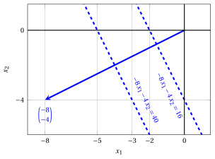
The figure shows:

• The gradient evaluated at \(\begin{pmatrix} 0 \\ 0 \end{pmatrix}\): \(\nabla f\left(\begin{pmatrix} 0 \\ 0 \end{pmatrix}\right) =\begin{pmatrix} -8 \\[0.5ex] -4 \end{pmatrix}\) (blue arrow)

• Two level sets (blue dashed lines): \(-8 x_1 -4 x_2 = 16\) and \(-8 x_1 -4 x_2 = 40\)

Example 1.3: graphs of linear functions

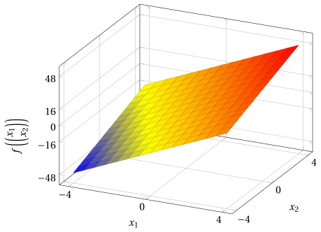
With \({\boldsymbol c}=\begin{pmatrix} 8\\ 4 \end{pmatrix}\), we have \(f\left(\begin{pmatrix} x_1 \\ x_2 \\ \end{pmatrix}\right)=8\;x_1 + 4\;x_2\). Its graph is:

Example 1.4: graphs of linear functions

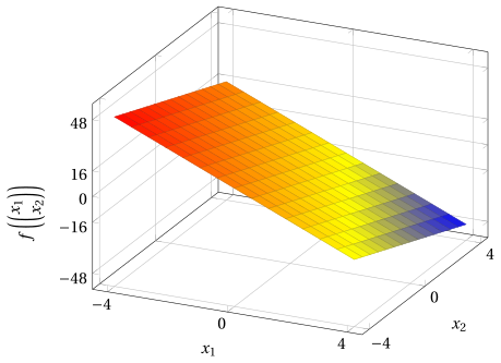
With \({\boldsymbol c}=\begin{pmatrix} -8\\ -4 \end{pmatrix}\), we have \(f\left(\begin{pmatrix} x_1 \\ x_2 \\ \end{pmatrix}\right)=-8\;x_1- 4\;x_2\). Its graph is:

Interactive lab

The ideas of the chapter, hands on: move the sliders and drag the points. Each app also opens full page in the interactive lab: Level lines.